Surface Waves Simulation: Dynamic Waveforms and Geometric Construction

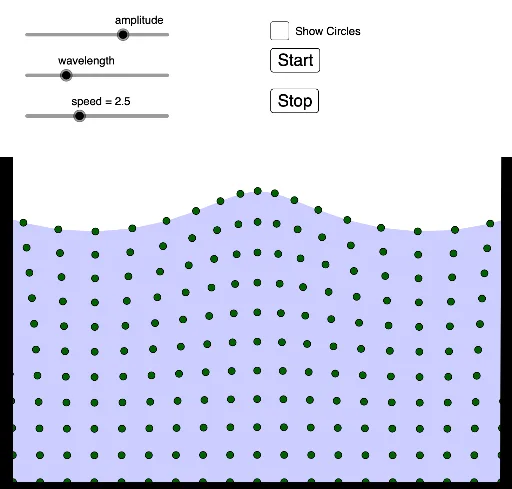
This example demonstrates a dynamic simulation of surface waves, using sliders to control amplitude, wavelength, and speed, visually showing wave propagation and superposition on a plane. Core mathematical concepts involve wave equations, trigonometric functions (sine/cosine) periodicity, parametric equations, and surface representation in differential geometry. Construction highlights: the Sequence command generates a series of points, Polygon builds polygonal patches, and Point defines key control points; objects include amplitude, wavelength, time parameter t, speed, and buttons (button1, button2) for start/reset animation; numerous named objects (A, B, C, D, a, poly1, f, g, h, etc.) build complex geometric relations, with sliders dynamically updating the waveform. Suitable for high school to university-level math or physics teaching, to understand waves, periodic functions, and parametric surface visualization, and as a reference for advanced GeoGebra interactive design.