
Surface Area by Pappus Theorem
Loading the math board and drawing, please wait…
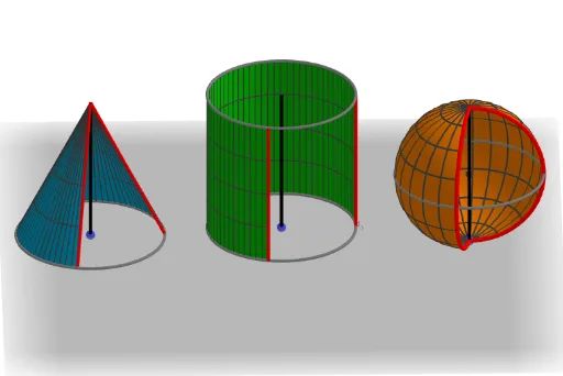
This example demonstrates the calculation of surface area of solids of revolution using Pappus' Theorem. Key math concepts include Pappus' Theorem, surface area of solids, and geometric transformations. Construction involves commands like Sequence, Polygon, Centroid, Circle, Conic, Segment, Midpoint, Vector, Line, CircleArc, Surface, Rotate, CircumcircleArc to visualize and apply the theorem. Suitable for high school students and math enthusiasts studying solid geometry and applications of Pappus' Theorem.
GeoGebra Commands & Parameters
Sequence(Rotate[A + (r, 0), i, A], i, ((-pi)) / 2, pi / 2, (2 * pi / n)) → l1Polygon(l1) → poly1Centroid(poly1) → BPolygon(E, G, F, D) → q1, e, g, f, dPolygon(J, K, I) → t1, i, j, kCircle(A, r) → cConic(K, D_1, Z, C_1, P) → hConic(F, E_1, B_1, A_1, Q) → pConic(S, G, J_1, W, V) → qConic(T, H_1, G_1, U, I_1) → r_2Segment(V, A_1) → lSegment(J, C_1) → mCentroid(q1) → K_1Centroid(t1) → L_1Midpoint(N_1, O_1) → T_1Midpoint(P_1, Q_1) → U_1Midpoint(R_1, S_1) → V_1Vector(T_1, O_1) → uVector(T_1, N_1) → vVector(U_1, Q_1) → wVector(U_1, P_1) → aVector(V_1, S_1) → bVector(V_1, R_1) → sSegment(K, O_1) → tSegment(I, N_1) → f_1Segment(D, P_1) → g_1Segment(F, Q_1) → h_1Segment(M, R_1) → i_1Segment(H_1, S_1) → j_1Segment(L_1, W_1) → k_1Midpoint(P, W_1) → Z_1Vector(P, W_1) → u_1Vector(Z_1, P) → v_1Midpoint(Q, A_2) → B_2Midpoint(A, B) → C_2Midpoint(M_1, L_1) → D_2Midpoint(C, K_1) → E_2Segment(M_1, L_1) → m_1Line(N, zAxis) → p_1Line(F_1, zAxis) → q_1Line(F_2, zAxis) → r_1Circle(N, r, p_1) → c_1Polygon(G_2, N, H_2) → t2, h_2, g_2, n_2Circle(F_1, r, q1) → d_1Circle(J_2, r, q1) → e_1Polygon(J_2, L_2, K_2, F_1) → q2, j_2, l_2, k_2, s_1Line(N_2, yAxis) → t_1Sequence(Rotate[N_2 + (r, 0), i, t_1], i, ((-pi)) / 2, pi / 2, (2 * pi / n)) → l2Polygon(l2) → poly2Circle(N_2, r, r_1) → c_2CircleArc(A, M, L) → d_2Segment(I, J) → l_1Segment(E, D) → n_1Segment(M, L) → f_2Segment(H, I_2) → i_2Segment(A, O_2) → p_2Segment(C, M_2) → m_2Surface(n_2, Rotation, p_1) → a_1Rotate(H_2, Rotation, p_1) → P_2Rotate(G_2, Rotation, p_1) → Q_2Segment(P_2, Q_2) → q_2Circle(N, r, p_1) → e_2Surface(l_2, Rotation, q_1) → b_1Rotate(L_2, Rotation, q_1) → R_2Rotate(K_2, Rotation, q_1) → S_2Segment(R_2, S_2) → s_2CircumcircleArc(U_2, T_2, F_2) → t_2Rotate(t_2, Rotation, r_1) → c_3Surface(t_2, Rotation, r_1) → w_1Segment(U_2, F_2) → a_2Segment(J_2, F_1) → b_2Segment(N, G_2) → f_3Sequence(I + ((r * cos(i)), (r / 3 * sin(i))), i, 0, (2 * pi), (2 * pi / 20)) → l3Segment(J, Element[l3, dd]) → g_3Sequence(D + ((r * cos(i)), (r / 3 * sin(i))), i, 0, (2 * pi), (2 * pi / 20)) → l4Sequence(E + ((r * cos(i)), (r / 3 * sin(i))), i, 0, (2 * pi), (2 * pi / 20)) → l5Segment(Element[l4, dd], Element[l5, dd]) → h_3Sequence(A + ((r * cos(i)), (r / 3 * sin(i))), i, 0, (2 * pi), (2 * pi / 20)) → l6CircumcircleArc(L, Element[l6, dd], M) → d_3
AI Drawing Prompt Reference
Visualize the calculation of surface area for solids of revolution using Pappus' Theorem. Start by drawing a rotating curve, then generate the solid through rotations and geometric transformations, highlighting key points like centroids and vertices. Include auxiliary lines and circles to demonstrate the theorem's application, and present the surface and volume calculations of the solid.
The prompt above was compiled from the original drawing commands and is for reference only.