
Stereographic Projections of Common Functions
Loading the math board and drawing, please wait…
In collections
surface 3D /3D-Oberflächen 1
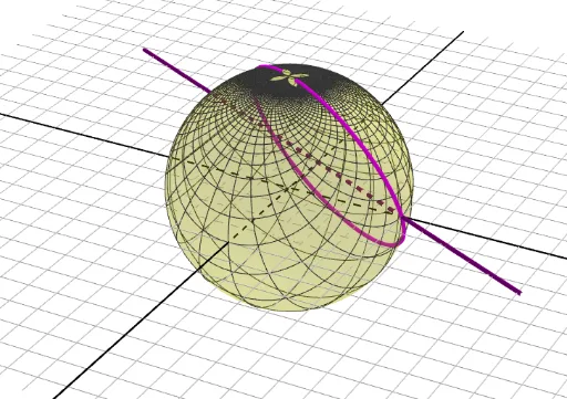
This example demonstrates the stereographic projections of common functions, showcasing geometric transformations and mappings. Key math concepts include spherical geometry, function representation, and coordinate geometry. Constructed using commands like Sphere, Sequence, SelectedElement, CurveCartesian, and Line in GeoGebra, it is suitable for high school and above students exploring the intersection of functions and geometry.
GeoGebra Commands & Parameters
Sphere((0, 0, 0), 1) → aSequence(Line[(w, 0, 0), (w, 1, 0)], w, -10, 10, 0.25) → L_3Sequence(Line[(0, w, 0), (1, w, 0)], w, -10, 10, 0.25) → L_4Sequence(IntersectPath[Plane[N, Line[(0, w, 0), (1, w, 0)]], a], w, -8, 8, 0.25) → L_1SelectedElement(L_5) → fSequence(IntersectPath[Plane[N, Line[(w, 0, 0), (w, 1, 0)]], a], w, -8, 8, 0.25) → L_2CurveCartesian(((2 * u / (1 + u^(2) + f(u)^(2))), (2 * f(u) / (1 + u^(2) + f(u)^(2))), (-1 + u^(2) + f(u)^(2)) / (1 + u^(2) + f(u)^(2))), u, -10, 10) → bLine((0, 0, 0), (1, 0, 0)) → gLine((0, 0, 0), (0, 1, 0)) → h