
Step Through Basic Statistics with TI 83/84 Calculator
Loading the math board and drawing, please wait…
In collections
Statistics Step Through Applets
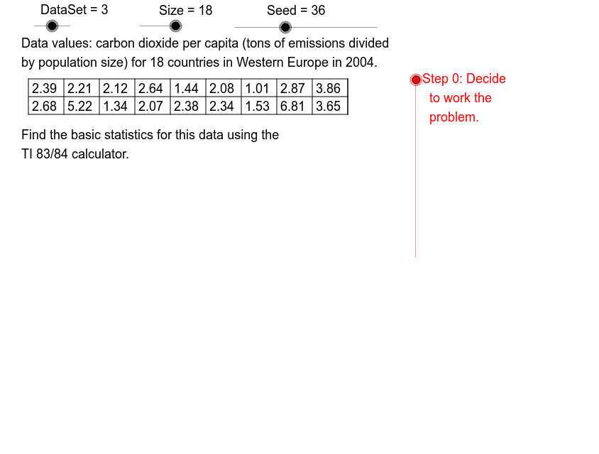
This example demonstrates the steps to compute basic statistics using a TI 83/84 calculator. It involves core mathematical concepts like statistical characteristics, datasets, median, mode, quartiles, etc. The construction utilizes GeoGebra commands and objects such as Element, Sequence, Max, Min, KeepIf, TableText, Sort, CountIf, Segment, If, Polygon, Sum, Q1, Q3, Median, Mode. It is suitable for high school and above students learning statistical computation methods.
GeoGebra Commands & Parameters
Element(RateSq, Mod[Seed, 8] + 1) → RateSequence(Mod[(Rate * k) + Start, 20] + 1, k, 0, 19, 1) → OptSeqElement(DataSets, DataSet) → DataSet1Element(AcSq, DataSet) → Ac0Sequence(Element[DataSet1, Element[OptSeq, k]], k, 1, Size) → DataSet2Max(DataSet2) → maxXMin(DataSet2) → minXSequence(8.5 - (1.1 * k), k, 0, 2) → LHSeqSequence(k, k, 1, 19) → StartSqKeepIf(floor(20 / x) ≠ 20 / x, StartSq) → RlPrSqSequence(Element[DataSet2, k], k, RL1 + 1, Size) → DspRw2Sequence(Element[DataSet2, k], k, 1, RL1) → DspRw1TableText({DspRw1, DspRw2, "hr"}) → DataListElement(DscSq, DataSet) → DataDescTableText({DataSet2}, "hr") → DataLineSort(DataSet2) → SortDataCountIf(x > 0, RateSq) → RateNoSegment(TbL1, TbR1) → tbhl1Segment(TbL2, TbR2) → tbhl2Segment(TbL0, TbR0) → tbhl0CountIf(x ≠ (0, 0), DataSet1) → DataCntIf(Mod[Size, 2] ≟ 1, Segment[TbR1, TbR0], Segment[TbR2, TbR0]) → tbrgSort(DataSet2) → DataSet3Sequence((k - 0.375) / (Size + 0.25), k, 1, Size) → PPVSequence(k, k, 12, 18, 1) → SzSqSequence(Segment[(TbLf + (TbCW * k), TbTp), (TbLf + (TbCW * k), TbBt)], k, 0, floor(Size / 2)) → TbVLinesSegment((DSL2, DST1), (DSL2, DSB)) → dsv1Segment((DSR1, DST1), (DSR1, DSB)) → dsv2Segment((DSL1, DST2), (DSR2, DST2)) → dsh1Segment((DSL1, DSB), (DSR2, DSB)) → dsh2Polygon(ARUL, ARLL, ARLR, ARUR) → ARbx, arul, arll, arlr, arurPolygon(BRUL, BRLL, BRLR, BRUR) → BRbx, brul, brll, brlr, brurPolygon(CRUL, CRLL, CRLR, CRUR) → CRbx, crul, crll, crlr, crurSum(DataSet2) → ΣxSequence(Element[DataSet2, k]^(2), k, 1, Size) → XsqSqQ1(DataSet2) → QLoQ3(DataSet2) → QHiMedian(DataSet2) → MedIf(Ac1 ≟ 1, ".", "s.") → PlTxtPolygon(DRUL, DRLL, DRLR, DRUR) → DRbx, drul, drll, drlr, drurPolygon(ERUL, ERLL, ERLR, ERUR) → ERbx, erul, erll, erlr, erurSegment(AAT, AAH) → aasSegment(AAL, AAH) → aalSegment(AAR, AAH) → aarSegment(BAH, BAT) → basSegment(BAL, BAH) → balSegment(BAR, BAH) → barSegment(CAT, CAH) → casSegment(CAL, CAH) → calSegment(CAR, CAH) → carElement(DataSet2, 6) → EnVlPolygon(FRUL, FRLL, FRLR, FRUR) → FRbx, frul, frll, frlr, frurMode(DataSet2) → DataModeSequence(Text[Element[OldData, k], (0.5, 6.1 - (0.5 * k))], k, 1, 7) → DsOldDtSequence(Text[Element[DataSet2, k], (0.5, 6.1 - (0.5 * k))], k, 1, 5) → DsNewDtSequence(Text[Element[DataSet3, k], (0.5, 6.1 - (0.5 * k))], k, 1, 7) → DsOrdDtSequence(Text[Element[DspRw1, k], (TbLf - 0.9 + (k * TbCW), TbTp - 0.4)], k, 1, RL1) → TbDtR1Sequence(Text[Element[DspRw2, k], (TbLf - 0.9 + (k * TbCW), TbTp - 0.4 - TbRH)], k, 1, RL2) → TbDtR2
AI Drawing Prompt Reference
Create a statistical chart demonstrating the process of computing basic statistics with a calculator. Include datasets, maximum and minimum values, quartiles, median, and mode. First plot the dataset, then mark the maximum and minimum values. Use different colors or lines to represent quartiles, median, and mode. Finally, display the dataset and calculation results in a table.
The prompt above was compiled from the original drawing commands and is for reference only.