
Staggered Hypocycloids: Parametric Curve Construction
Loading the math board and drawing, please wait…
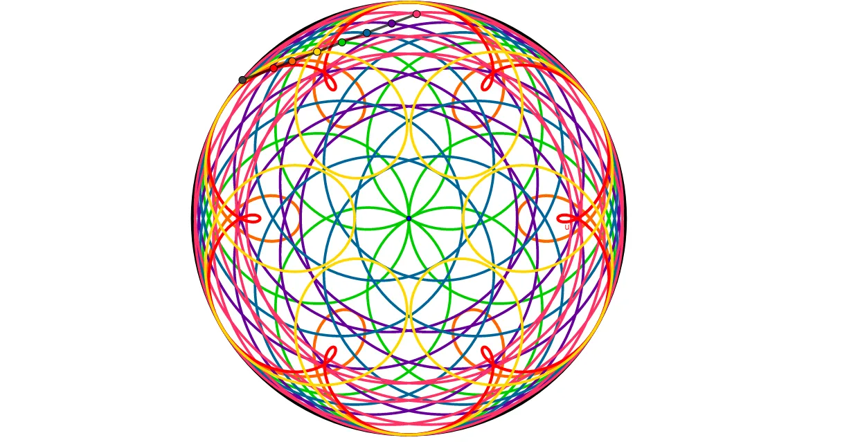
This example demonstrates how staggered hypocycloid curves can be generated by combining rotating circles, intersection points, and a controlled sequence of offsets, producing a family of continuous but shifted curve shapes. The key math concepts are parametric curve representation, the periodic nature of trigonometric functions, and hypocycloid-style geometry arising from relative rotation/rolling mechanisms. Construction focuses on building the required geometric elements using GeoGebra commands such as Line, Circle, Intersect, Point, Rotate, Ray, Segment, Midpoint, and CurveCartesian. Parameters like t (the running parameter), radii (e.g., R), angular speed (w), and derived quantities (e.g., w1, a, n) control the rotation and staggering so that points like A, B, B′, C, C′, I, I′, and H act as anchors. Finally, the tracked locus is plotted in Cartesian coordinates via CurveCartesian to render the staggered hypocycloid graph. Suitable for high school to undergraduate lessons on parametric equations, trigonometry-based modeling, and geometric transformation/trajectory construction.
GeoGebra Commands & Parameters
Line(A, xAxis) → nCircle(A, R) → cIntersect(c, n) → E, FPoint(c) → BRotate(F, (t * w), A) → B'Ray(A, B') → aSegment(A, B') → jRay(A, B') → fMidpoint(B', A) → LCircle(L, B') → rRotate(A, (w1 * t), L) → A'Segment(L, A') → gCurveCartesian(x(A) + (R / 2 * cos((w * i))) - (R / 2 * cos(((w1 + w) * i))), y(A) + (R / 2 * sin((w * i))) - (R / 2 * sin(((w1 + w) * i))), i, 0, t) → oMidpoint(B', L) → DCircle(D, L) → eRotate(L, (w1 * t), D) → L'CurveCartesian(x(A) + ((3 * R / 4) * cos((w * i))) - (R / 4 * cos(((w1 + w) * i))), y(A) + ((3 * R / 4) * sin((w * i))) - (R / 4 * sin(((w1 + w) * i))), i, 0, t) → hMidpoint(L, A) → HCircle(H, B') → sRay(H, A) → f_1Intersect(s, f_1) → I,Rotate(I, (w1 * t), H) → I'Midpoint(I, A) → CMidpoint(C, B') → JCircle(J, C) → dCurveCartesian(x(A) + (Distance[H, A] * cos((w * i))) - (Distance[H, B'] * cos(((w1 + w) * i))), y(A) + (Distance[H, A] * sin((w * i))) - (Distance[H, B'] * sin(((w1 + w) * i))), i, 0, t) → iCurveCartesian(x(A) + (Distance[A, J] * cos((w * i))) - (Distance[J, B'] * cos(((w1 + w) * i))), y(A) + (Distance[A, J] * sin((w * i))) - (Distance[J, B'] * sin(((w1 + w) * i))), i, 0, t) → bRotate(C, (w1 * t), J) → C'Rotate(I, (w1 * t), H) → I'_{1}Midpoint(B', J) → KIntersect(c, f_1) → M,Midpoint(M, I) → NMidpoint(B', H) → OCircle(O, H) → c_1Midpoint(B', N) → PCircle(P, N) → d_1CurveCartesian(x(A) + (Distance[A, P] * cos((w * i))) - (Distance[P, B'] * cos(((w1 + w) * i))), y(A) + (Distance[A, P] * sin((w * i))) - (Distance[P, B'] * sin(((w1 + w) * i))), i, 0, t) → vMidpoint(B', K) → QCircle(Q, K) → kCurveCartesian(x(A) + (Distance[A, Q] * cos((w * i))) - (Distance[Q, B'] * cos(((w1 + w) * i))), y(A) + (Distance[A, Q] * sin((w * i))) - (Distance[Q, B'] * sin(((w1 + w) * i))), i, 0, t) → uRotate(N, (w1 * t), P) → N'CurveCartesian(x(A) + (Distance[A, O] * cos((w * i))) - (Distance[O, B'] * cos(((w1 + w) * i))), y(A) + (Distance[A, O] * sin((w * i))) - (Distance[O, B'] * sin(((w1 + w) * i))), i, 0, t) → lRotate(H, (w1 * t), O) → J'Rotate(K, (w1 * t), Q) → K'Segment(N', B') → g_1
AI Drawing Prompt Reference
Draw a family of staggered hypocycloids by combining rotating circles, intersection points, and controlled offsets to create continuous but shifted curve shapes. Start with a line and a circle, find their intersections, then rotate one intersection point to form rays and segments. Locate midpoints, draw new circles, and rotate points on the original circle, tracking their paths. Use parametric equations incorporating trigonometric periodicity and geometric transformations to plot the locus, resulting in a series of interlocking, offset curves.
The prompt above was compiled from the original drawing commands and is for reference only.