
Sphere: generate two uniformly scattered points from one uniform source (Icosahe
Loading the math board and drawing, please wait…
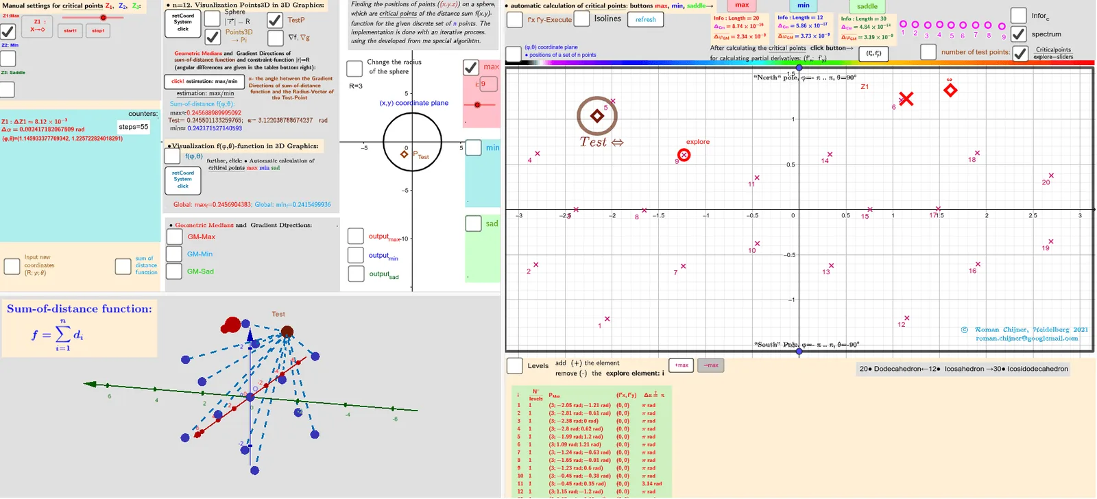
This example demonstrates how to obtain two different points on a sphere that are as uniformly separated as possible by using a single underlying uniform random distribution, using an icosahedron-based reference with V=12. Visually, it focuses on producing two points whose mutual spacing on the spherical surface is maximized according to a chosen score. Key math ideas include spherical geometry (Sphere/Surface), vector/coordinate representation, mapping parameters to the sphere, measuring angular/Euclidean separation (Angle, Length), and selecting the best pair via evaluation functions and extremum logic (If, Min/Max). In construction, candidate points are generated and represented as vectors on/relative to a Sphere, then their relationship is computed using Angle and distance. A scoring function (built with Function and optionally aggregation like Sum) is evaluated and filtered: If constraints are met, the pair that optimizes the objective is selected (via Min/Max with tolerance parameters). The GeoGebra setup leverages commands/objects such as Sphere, Circle, Vector, Angle, Length, Function, If, Max, Min, Polygon/PolyLine for geometry display, and TableText/Textfield for reporting intermediate results, along with text/annotation utilities (e.g., RotateText). Suitable for high school to early university instruction in geometry, computational visualization, and introductory probabilistic sampling concepts.
GeoGebra Commands & Parameters
Polygon({((-π), ((-π)) / 2), ((-π), π / 2), (π, π / 2), (π, ((-π)) / 2)}) → q_2PointIn(q_2) → Atest_2Function(f01, (-π), π, ((-π)) / 2, π / 2) → f0Zip((x(a), y(a), f0(a)), a, Zmin_2) → fmin3DZip((x(a), y(a), f0(a)), a, Zmax_2) → fmax3DVector((1.3 * Z3), (1.5 * Z3)) → AVZ3rVector((1.3 * Z3), (1.3 * Z3) + UnitVector[Sum[Zip[UnitVector[a - Z3], a, lP]]]) → AVZ3Vector((1.3 * Z2), (1.5 * Z2)) → AVZ2rVector((1.3 * Z2), (1.3 * Z2) + UnitVector[Sum[Zip[UnitVector[a - Z2], a, lP]]]) → AVZ2Vector((1.3 * Z1), (1.5 * Z1)) → AVZ1rVector((1.3 * Z1), (1.3 * Z1) + UnitVector[Sum[Zip[UnitVector[a - Z1], a, lP]]]) → AVZ1Vector((1.3 * Atest_R), (1.3 * Atest_R) + UnitVector[Sum[Zip[UnitVector[a - Atest_R], a, lP]]]) → AVtestVector((1.3 * Atest_R), (1.5 * Atest_R)) → AVtestrSphere(O, R) → spheraCircle(O, R, xOyPlane) → cPointIn(q_2) → RZ1_2PointIn(q_2) → RZ2_2Angle(AVtest, AVtestr) → αAAngle(AVZ1, AVZ1r) → αZ1Angle(AVZ2, AVZ2r) → αZ2Zip(Segment[Atest_R, p], p, lP) → segSum(seg) → sum_segPolyLine({((-π), ((-π)) / 2), ((-π), π / 2), (π, π / 2), (π, ((-π)) / 2), ((-π), ((-π)) / 2)}) → q1Flatten(Sequence[Sequence[((-π) + ((2 * π / na) * i), ((-π)) / 2 + (π / na * j)), j, 1, na], i, 1, na]) → ltest_2Zip((R; x(a); y(a)), a, ltest_2) → ltest_3Length(lZmax') → lälZmax'Textfield(n) → InputBox11alfa(R, lP, lZsad') → αsadIf(αZ1 > 100°, 180° - αZ1, αZ1) → αZ1'Textfield(m_1) → InputBox12Textfield(t) → InputBox13Textfield(m_2) → InputBox14PointIn(q_2) → RZ3_2Sum(Zip[1 / Length[p - Z3], p, lP]) → ZahZ3Angle(AVZ3, AVZ3r) → αZ3Textfield(R) → InputBox1Textfield(na) → InputBox2Max(f(Zmax_2)) → max_fMin(f(Zmin_2)) → min_fZip(Text["d_{" + (a) + "}", (Atest_R + Element[lP, a]) / 2], a, 1…n) → lPtxtZip(Segment[F_o, p], p, lP) → seg0Sum(seg0) → sum_seg0RotateText(txt, 90°) → txt1Sum(lZ3sad) → sumlZ3sadTextfield(Points3D) → InputBox7Textfield(lZsad') → InputBox17Textfield(lZmin') → InputBox16Textfield(lZmax') → InputBox15Textfield(jmin) → InputBox18Textfield(jmax) → InputBox19Textfield(jsad) → InputBox20Zip(Text["" + (b), a - (0.1, 0.1)], a, Zmax_2, b, 1…Length[Zmax_2]) → l2maxtxtZip(Text["" + (b), a - (0.1, 0.1)], a, Zmin_2, b, 1…Length[Zmin_2]) → l2mintxtZip(Text["" + (b), a - (0.1, 0.1)], a, Zsad_2, b, 1…Length[Zsad_2]) → l2sadtxtZip(Vector[r1, (1.153846154 * r1)], r1, (1.3 * Zip[(R * UnitVector[a]), a, lZmax'])) → lVmaxrZip(Vector[r1, (1.153846154 * r1)], r1, (1.3 * Zip[(R * UnitVector[a]), a, lZmin'])) → lVminrZip(Vector[r1, (1.153846154 * r1)], r1, (1.3 * Zip[(R * UnitVector[a]), a, lZsad'])) → lVsadralfa(R, lP, lZmax') → αmaxalfa(R, lP, lZmin') → αminarrow(R, lP, lZmax') → lVmaxarrow(R, lP, lZmin') → lVminarrow(R, lP, lZsad') → lVsadCurveCartesian((-π) + ((2 * π) * a), ((-π)) / 2, f0((-π) + ((2 * π) * a), ((-π)) / 2), a, 0, 1) → par1CurveCartesian((-π) + ((2 * π) * a), π / 2, f0((-π) + ((2 * π) * a), π / 2), a, 0, 1) → par2CurveCartesian((-π), ((-π)) / 2 + (π * a), f0((-π), ((-π)) / 2 + (π * a)), a, 0, 1) → par3CurveCartesian(π, ((-π)) / 2 + (π * a), f0(π, ((-π)) / 2 + (π * a)), a, 0, 1) → par4Polygon({((-π), ((-π)) / 2), ((-π), π / 2), (π, π / 2), (π, ((-π)) / 2)}) → q_3Zip((x(a), y(a), f0(a)), a, Zsad_2) → fsad3DTextfield(achs) → InputBox3Zip(Atest_2 + (r_c; ((2 * π / n_c) * k)), k, 0…(n_c - 1)) → l0rSum(Unique[sgn(f(Atest_2) - f(l0r))]) → sum_rSum(Sequence[If[sum00_r(i) ≠ sum00_r(i + 1), 1, 0], i, 1, Length[sum00_r] - 1]) → sum01_rCircle(Atest_2, 0.2) → ciTableText(Append["i", Sequence[Length[lZsad']]], Append["\frac{N°}{levels} ", msad], Append["P_{sad }", lZsad'], Append["(f'x,f'y)", lZf'xysad], Append[" Δα≟ π ", αsad], "v") → text2cTableText(Append["i", Sequence[Length[αmax]]], Append["\frac{N°}{levels} ", mmax], Append["P_{Max }", lZmax'], Append["(f'x,f'y)", lZf'xymax], Append[" Δα≟ π ", αmax], "v") → text2aTableText(Append["i", Sequence[Length[αmin]]], Append["\frac{N°}{levels} ", mmin], Append["P_{Min }", lZmin'], Append["(f'x,f'y)", lZf'xymin], Append[" Δα≟ π ", αmin], "v") → text2b
AI Drawing Prompt Reference
Create a 3D sphere with a defined center and radius. Generate a set of candidate points on its surface by parameterizing a reference region and mapping those parameters onto the sphere; represent each candidate by its position vector from the center. Sample additional candidates using the same underlying uniform source idea, then choose a pair of points whose mutual separation on the spherical surface is as large as possible according to an evaluation based on angular separation (via the angle between their center-to-point vectors) and distance/length-derived measures. Display the two selected points through their direction vectors, show the corresponding angle measurement with text, and include auxiliary polylines or line segments that visualize the reference region and the selected directions.
The prompt above was compiled from the original drawing commands and is for reference only.