
Speed vs Height Simulation
Loading the math board and drawing, please wait…
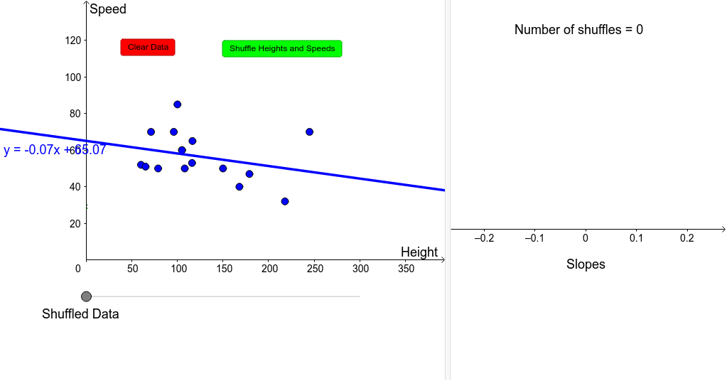
This example demonstrates the relationship between speed and height through scatter plots and linear fitting. It involves core math concepts like real numbers, definite integral, tangent line, confidence interval, and unit circle. Construction highlights include using GeoGebra commands such as Shuffle, Sequence, FitLineY, Slope, DotPlot, Sort, Segment, Point, and If, with objects like Heights, Speeds, and slopes. Suitable for high school and above in probability & statistics and calculus introductory lessons.
GeoGebra Commands & Parameters
Shuffle(Heights) → ShuffledHeightsShuffle(Speeds) → ShuffledSpeedsSequence((Element[ShuffledHeights, i], Element[ShuffledSpeeds, i]), i, 1, 16) → list1FitLineY(list1) → aSlope(a) → mDotPlot(slopes, true) → list2FitLineY(list3) → bSort(Heights) → sortheightsSort(Speeds) → sortspeedsSequence((Element[sortheights, i], Element[sortspeeds, i]), i, 1, 16) → list4FitLineY(list4) → eSegment(Q, R) → fPoint(list5) → SIf(x(S) < 100, "Shuffled Data", If[x(S) > 250, "Greatest Slope", "Original Data"]) → text2DotPlot(original, true) → list6DotPlot(best, true) → list7
AI Drawing Prompt Reference
Plot a scatter plot to show the relationship between speed and height, using shuffled height and speed data to generate the scatter plot, then use linear fitting to get the slope and plot a histogram of the slopes. Sort the heights and speeds, generate another scatter plot and perform linear fitting. Finally, display different text based on the position of the points.
The prompt above was compiled from the original drawing commands and is for reference only.