Solving Systems of Equations by Substitution: Dynamic Intersection Demo

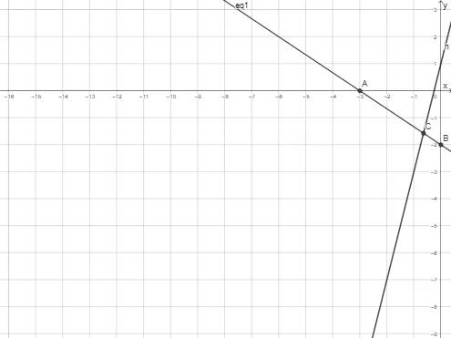
① This GeoGebra example dynamically demonstrates the complete process of solving a system of two linear equations using the substitution method, visually showing that the intersection point of the two lines (or curves) is exactly the solution of the system. ② Core mathematical concepts include: solutions of equation systems, substitution/elimination method, intersection of function graphs, and the geometric meaning of roots (Root) and intersections (Intersect). ③ Construction highlights: from the construction summary, the Solve command is used to directly solve the system, Root finds the roots of equations, and Intersect computes the intersection points of the two function graphs; objects include function h, equation eq1, line l2, points A, B, text1, and point C, with text displaying the solving steps and results. ④ Suitable for middle and high school students learning algebra and coordinate geometry, to understand the principle of solving systems by substitution and the correspondence between algebraic solutions and geometric intersections, also useful as an interactive classroom demonstration tool.