
Law of Large Numbers Demo
Loading the math board and drawing, please wait…
In collections
Introduction to Probability
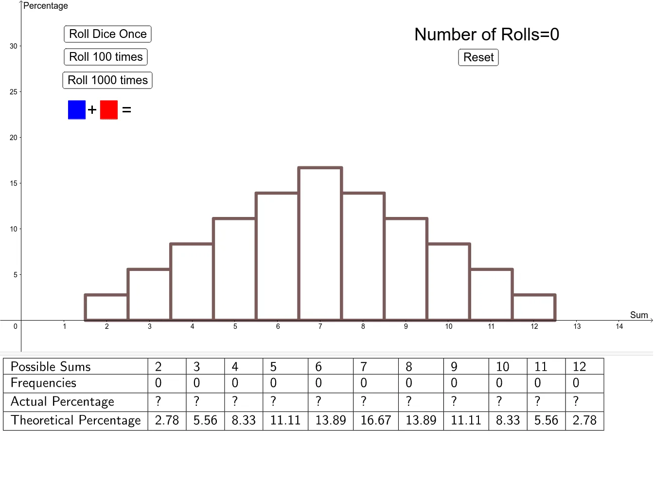
This example demonstrates how empirical probabilities converge towards theoretical probabilities as the number of trials increases, illustrating the Law of Large Numbers in Probability & Statistics. It uses GeoGebra commands like Polygon, Append, TableText, and Histogram for visualization. Suitable for high school and above, focusing on probability concepts and experimental design.
GeoGebra Commands & Parameters
Polygon({(1.1, 22), (1.1, 24), (1.5, 24), (1.5, 22)}) → poly1Polygon({(1.85, 22), (1.85, 24), (2.25, 24), (2.25, 22)}) → poly2Append("Frequencies", sums) → TsumsAppend("Theoretical Percentage", (thProb * 100)) → TthProbAppend("Actual Percentage", (probs * 100)) → TprobsAppend("Possible Sums", PossibleSums) → TpossibleTableText({Tpossible, Tsums, Tprobs, TthProb}, "|_") → text5Histogram(classes, (probs * 100)) → ExHistHistogram(classes, (thProb * 100)) → ThHist
AI Drawing Prompt Reference
Create a graph demonstrating the Law of Large Numbers, including a rectangle representing possible sums, and histograms for actual and theoretical percentages. First, draw the rectangle for possible sums, then plot the histograms for actual and theoretical percentages, and finally display the frequency table.
The prompt above was compiled from the original drawing commands and is for reference only.