
Solving Similar Triangles
Loading the math board and drawing, please wait…
In collections
Similar Triangles Review
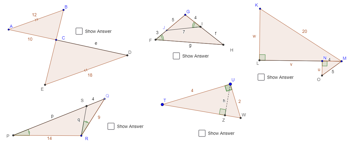
This example demonstrates the construction and analysis of similar triangles using GeoGebra. It involves core mathematical concepts such as the criteria and properties of similar triangles, trigonometric function applications, angle measurement, and segment ratio relationships. The construction utilizes commands and objects like Circle, Point, Ray, Polygon, Intersect, Line, Segment, Angle, OrthogonalLine, and Midpoint. It is suitable for high school mathematics education, aiding students in visually understanding the geometric properties and problem-solving methods of similar triangles.
GeoGebra Commands & Parameters
Circle(A, c) → dCircle(A, b) → e_4Point(d) → BPoint(e_4) → CRay(A, C) → aRay(B, C) → f_4Polygon(A, B, C) → poly1, c_1, a_1, b_1Circle(C, c' / (c / b)) → kIntersect(k, a, 1) → DLine(D, c_1) → mIntersect(m, f_4) → EPolygon(C, D, E) → poly2, e_1, c_2, d_1Segment(C, D) → p_2Circle(G, i) → q_2Circle(G, j) → tPoint(q_2) → JCircle(J, g_3) → f_1Intersect(t, f_1, 1) → ISegment(J, G) → g_1Segment(G, I) → h_1Segment(I, J) → i_1Ray(G, J) → j_1Circle(J, fj) → k_1Intersect(k_1, j_1, 2) → FCircle(I, G) → p_1Intersect(p_1, i_1, 1) → H_1Circle(F, Radius[p_1]) → q_1Intersect(q_1, g_1, 1) → I_1Circle(I_1, Segment[H_1, G]) → r_1Intersect(q_1, r_1, 2) → K_1Ray(F, K_1) → l_1Ray(G, I) → m_1Intersect(l_1, m_1) → HPolygon(G, F, H) → poly3, h_2, g_2, f_2Angle(G, I, J) → αAngle(H, F, G) → βSegment(J, F) → h_{4}Point(h_{4}) → L_1Segment(F, H) → n_1Segment(I, H) → s_1Point(Circle[R, s]) → QSegment(R, Q) → t_1Circle(Q, r) → d_2Circle(R, q_4) → e_2Intersect(d_2, e_2, 2) → SCircle(R, q') → k_2Ray(Q, S) → a_2Intersect(k_2, a_2, 1) → PPolygon(P, R, Q) → poly4, q_3, n_2, r_2Segment(R, S) → b_2Angle(R, P, S) → γAngle(Q, R, S) → δSegment(S, Q) → i_2Segment(P, S) → j_2Segment(R, S) → qSegment(P, S) → pCircle(M, o) → s_2Circle(M, n) → t_2Point(s_2) → NSegment(M, N) → l_2OrthogonalLine(N, l_2) → m_2Intersect(t_2, m_2, 2) → OSegment(O, M) → a_3Polygon(M, N, O) → poly5, o_1, u, n_3Ray(M, N) → b_3Circle(M, l) → c_3Point(c_3) → KOrthogonalLine(K, b_3) → d_3Intersect(d_3, b_3) → LPolygon(M, L, K) → poly6, v, w, l_3Angle(O, N, M) → εAngle(M, L, K) → ζSegment(L, N) → e_3Segment(N, O) → f_3Segment(F, H) → gSegment(I, H) → fSegment(C, D) → eSegment(T, U) → h_3OrthogonalLine(U, h_3) → i_3Midpoint(T, U) → VCircle(U, V) → k_3Intersect(k_3, i_3, 1) → WPolygon(T, U, W) → t1, w_1, t_3, u_1Angle(T, U, W) → ηAngle(T, U, W) → θOrthogonalLine(U, u_1) → j_3Intersect(j_3, u_1) → ZSegment(U, Z) → hAngle(U, Z, T) → ιSegment(U, Z) → m_3