
Slope Fields
Loading the math board and drawing, please wait…
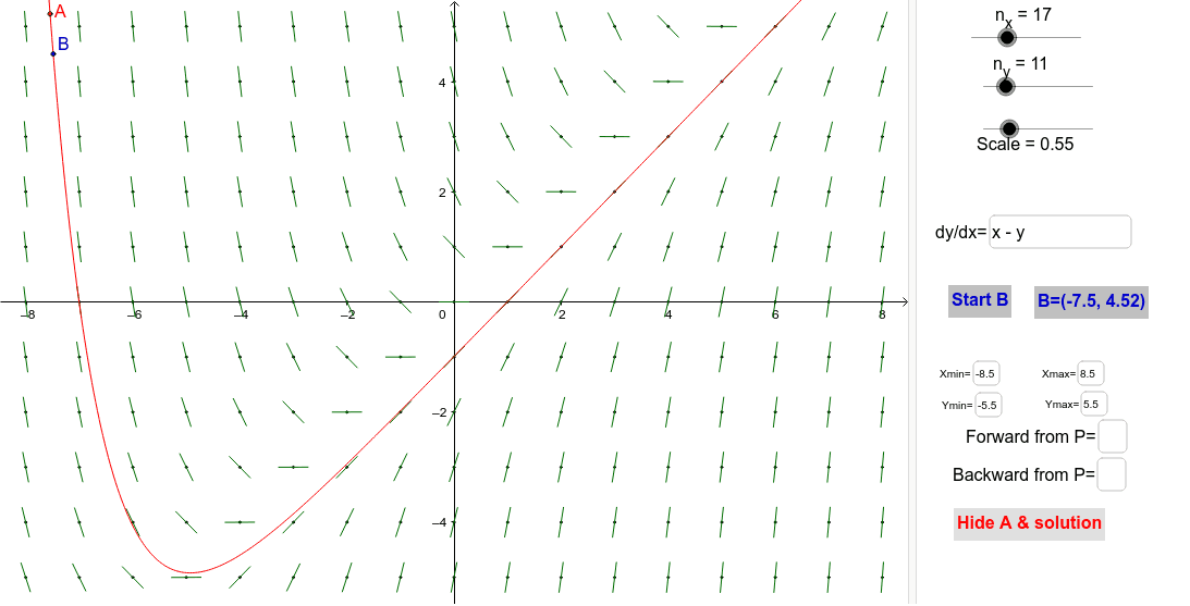
This example demonstrates the graphical representation of slope fields for differential equations, visually illustrating the distribution of solution curves. Core mathematical concepts include differential equations, derivatives, and integrals. It utilizes GeoGebra commands and objects such as Sequence, Join, Length, Textfield, SolveODE, If, and Point in its construction. Suitable for high school students and above, particularly for those studying calculus to understand the geometric meaning of differential equation solutions.
GeoGebra Commands & Parameters
Sequence(Sequence[(xStart + ((i - 0.5) * xStep), yStart + ((j - 0.5) * yStep)), i, 1, n_x], j, 1, n_y) → GP1Join(GP1) → GPLength(GP) → NPSequence(sqrt(1 + Element[slp, k]^(2)), k, 1, NP) → lenSequence(Segment[Element[GP, k] - ((Scale * 0.5) * (1, Element[slp, k]) / Element[len, k]), Element[GP, k] + ((Scale * 0.5) * (1, Element[slp, k]) / Element[len, k])], k, 1, NP) → SegsTextfield(f) → DYDXTextfield(Xmin) → xMinTextfield(Xmax) → xMaxTextfield(Ymin) → yMinTextfield(Ymax) → yMaxTextfield() → StartPointSolveODE(f, x(A), y(A), x(Corner[3]), Step) → ForwardATextfield() → BackwardSolveODE(f, x(A), y(A), x(Corner[4]), (-Step)) → BackAIf(togA ≟ 1, "Hide A & solution", "Show A & solution") → ShowAPoint(ForwardA) → BIf(togB ≟ 1, "Stop B", "Start B") → StartB
AI Drawing Prompt Reference
Draw a slope field for differential equations, showing the distribution of solution curves, including short arrows and text labels with lengths adjusted by slopes, covering a specified area, start by creating grid points, then draw arrows, and finally add example solution curves and labels to indicate the range.
The prompt above was compiled from the original drawing commands and is for reference only.