Slope Fields: Problem 2 – Visualizing Differential Equation Solutions

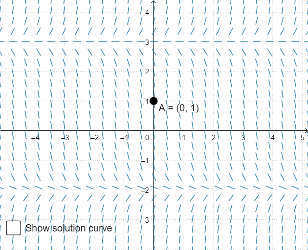
This GeoGebra example demonstrates the construction and interpretation of slope fields (direction fields) for a first-order differential equation, focusing on how solution curves align with the field. Core mathematical concepts include differential equations, slope fields, initial value problems, and the relationship between particular and general solutions. The construction uses GeoGebra commands SolveODE to compute symbolic/numeric solutions and SlopeField to generate the direction field. Key objects include a button (button1) for interactive control, function f, point A, solution curves Sol1 and Sol2, parameter a, and function F, allowing dynamic exploration of how changing initial conditions or parameters alters the solution trajectories. This resource is ideal for high school AP Calculus or introductory college calculus courses, helping students visualize existence, uniqueness, and the geometric intuition behind solving differential equations.