
Slope Fields: Problem 1
Loading the math board and drawing, please wait…
In collections
MATH1052-edX
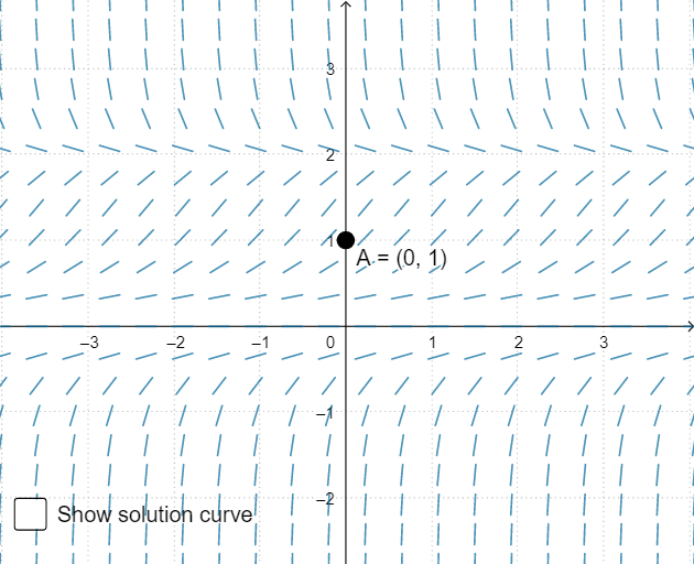
This example demonstrates how to visualize solutions to differential equations using slope fields. By plotting the slope field, one can intuitively understand the geometric meaning and dynamic behavior of the differential equation. Key math concepts involved include differential equations, vector fields, and geometry. The construction uses GeoGebra commands SolveODE and SlopeField to generate the slope field and solutions to the differential equation. Suitable for high school and introductory college students studying calculus and differential equations.
GeoGebra Commands & Parameters
SolveODE(f, x(A), y(A), 10, 0.01) → Sol1SolveODE(f, x(A), y(A), -10, 0.01) → Sol2SlopeField(f, 20, 0.7) → F
AI Drawing Prompt Reference
Create a slope field plot for the differential equation dy/dx = f(x,y). Choose a reference point, then compute and draw two solution curves passing through that point, extending forward and backward along the x‑direction. The slope field should consist of short line segments uniformly spaced (about a 20‑by‑20 grid) with length roughly 0.7, each segment indicating the slope given by the equation. Include the two solution curves together with the field to visualize the geometric behavior of the solutions.
The prompt above was compiled from the original drawing commands and is for reference only.