Slope Field with an ODE Solution Overlay (Slope Field 1)

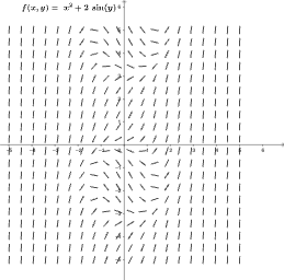
This example demonstrates how to visualize an initial value problem for a first-order differential equation by combining a slope field (direction field) with an overlaid numerical solution curve. The key ideas are the first-order ODE y' = f(x,y), slope field interpretation (the local tangent slope at each grid point), and solving an ODE under an initial condition to produce a specific trajectory. In GeoGebra, the construction relies on the commands SlopeField and SolveODE: SlopeField uses the function f together with parameters such as n (grid resolution) and l (view/range) to generate the direction field slopefield1; then SolveODE computes the solution based on an initial point P and outputs the solution curve g. A text object (text1) is used to label or describe the setup. Suitable for high school and early university instruction, as well as interactive exploration of ODE behavior.