Slope and Direction Field Plotter

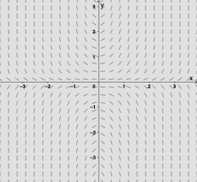
① This interactive GeoGebra example demonstrates how to plot the slope field (direction field) of a first-order differential equation and overlay numerical solution curves, revealing the behavior of solution families. ② Core mathematical concepts include differential equations, slope fields, direction fields, numerical integration (e.g., Euler or Runge-Kutta methods), initial value problems, and the geometric interpretation of solutions. ③ Construction highlights: using GeoGebra commands such as SolveODE to solve the ODE, SlopeField to generate the field, Sequence and Element to build grid points, Segment to draw direction segments, Textfield and InputBox for interactive input, sliders (scale, density, xstep, ystep) to adjust field density and range, and displaying numerical integrals (numericalIntegral1, numericalIntegral2) and solution curves. ④ Suitable for high school to university-level differential equations courses, math labs, or exploratory activities, helping students understand the relationship between slope fields and solution curves and how parameter changes affect solutions.