
Simpson's Rule Integration
Loading the math board and drawing, please wait…
In collections
Fun with Functions
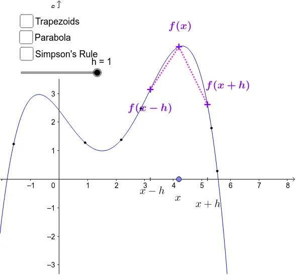
Simpson's Rule is a numerical integration method for approximating the area under a curve. This example demonstrates a single increment h width for Simpson's rule. The key mathematical concepts involve polynomial fitting and integral approximation. Construction uses GeoGebra commands like Polynomial, Point, Segment, and Integral. Suitable for high school students or college freshmen learning calculus basics.
GeoGebra Commands & Parameters
Polynomial({A, B, C, D, E, F}) → fPoint(xAxis) → Z_0Segment(F_m, F_0) → aSegment(F_0, F_p) → bPolynomial({F_m, F_0, F_p}) → gPolygon(Z_0, Z_p, F_p, F_0) → poly1, z_0, z_p, f_1, f_0Polygon(Z_m, Z_0, F_0, F_m) → poly2, d, k, l, mIntegral(g, xGm, xGp) → c
AI Drawing Prompt Reference
Draw a curve with two trapezoids below it approximating the area under the curve. One trapezoid connects the endpoints and a midpoint, the other connects the midpoint and endpoints, showing the region enclosed by the trapezoids and the curve to illustrate Simpson's Rule.
The prompt above was compiled from the original drawing commands and is for reference only.