
Simpson's Rule Example 2: Parabolic Approximation for Numerical Integration
Loading the math board and drawing, please wait…
This GeoGebra example demonstrates Simpson's Rule for numerical integration, where the interval is divided into an even number of subintervals and each pair is approximated by a quadratic parabola, yielding a more accurate estimate of the definite integral than the trapezoidal rule. Core mathematical concepts include definite integrals, numerical integration, parabolic interpolation, comparison with trapezoidal and rectangular sums, and error behavior. The construction uses GeoGebra commands such as TrapezoidalSum and RectangleSum to generate trapezoidal and rectangular approximations, Integral for the exact value, and Textfield for user inputs of endpoints a, b and number of subintervals n. Key objects include the function f1, trapezoids, midpoint, step size dx, current parabola currentParab, and all parabolas allParabs, with buttons to toggle the Simpson sum, show parabolas, and cycle through them. This is ideal for high school or college calculus courses to visually illustrate why Simpson's Rule often outperforms the trapezoidal rule.
GeoGebra Commands & Parameters
TrapezoidalSum(f, a, b, n) → trapezoidsRectangleSum(f, a, b, n, 0.5) → midpointIntegral(f, a, b) → geogebraTextfield(f1) → foffxTextfield(a) → setaTextfield(b) → setbTextfield(n) → inputn
AI Drawing Prompt Reference
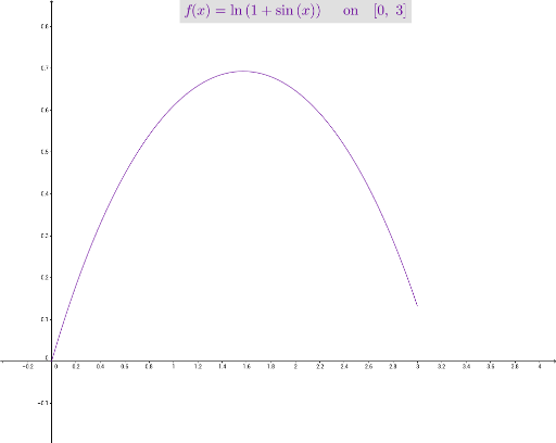
Draw the graph of function f1 in the interval [a, b], and divide it into n subintervals. Calculate and display the integral approximations using the trapezoidal and midpoint rules. Then, approximate the integral of each subinterval with a parabola and display all the parabolas. Finally, calculate and show the exact integral value to compare the accuracy of these methods.
The prompt above was compiled from the original drawing commands and is for reference only.