
Second Order Linear DE Solver
Loading the math board and drawing, please wait…
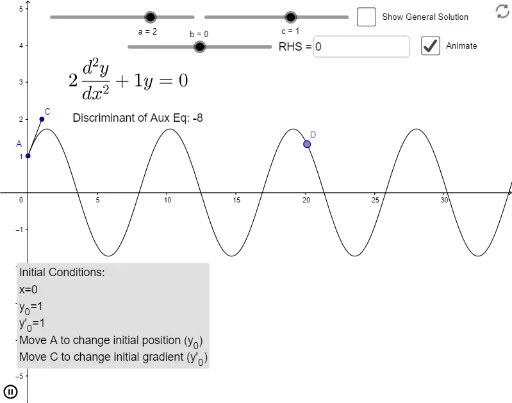
This example demonstrates solving second order linear differential equations in real-time by adjusting coefficients. Key mathematical concepts include second order differential equations, derivatives, and integrals. GeoGebra commands such as SolveODE, Textfield, and CurveCartesian are used. Suitable for calculus and advanced mathematics courses.
GeoGebra Commands & Parameters
Corner(2) → c2Point(j) → CLine(A, C) → lSlope(l) → mOrthogonalLine(B, xAxis) → eSegment(A, C) → sSolveODE(b / a, c / a, f(x) / a, x(A), y(A), m, x(B), 0.001) → numericalIntegral1Textfield(f) → InputBox1Corner(1) → c1Corner(3) → c3Corner(4) → c4Corner(2, 1) → C1Corner(2, 2) → C2Corner(2, 3) → C3Corner(2, 4) → C4Point(numericalIntegral1) → DCurveCartesian((0.5 * sin(((16 * π / (4 - y(E))) * (tt - y(E))))), tt, tt, y(E), 4) → kIf(b ≟ 0, text5, text1) → DEeq
AI Drawing Prompt Reference
Draw a graph demonstrating the real-time solution of second-order linear differential equations by adjusting coefficients. Start with a baseline and a point, then calculate the slope and draw a perpendicular line. Solve the differential equation to get a numerical integral result and determine a point using it. Finally, plot the solution curve based on the input function and display the equation depending on the coefficients.
The prompt above was compiled from the original drawing commands and is for reference only.