
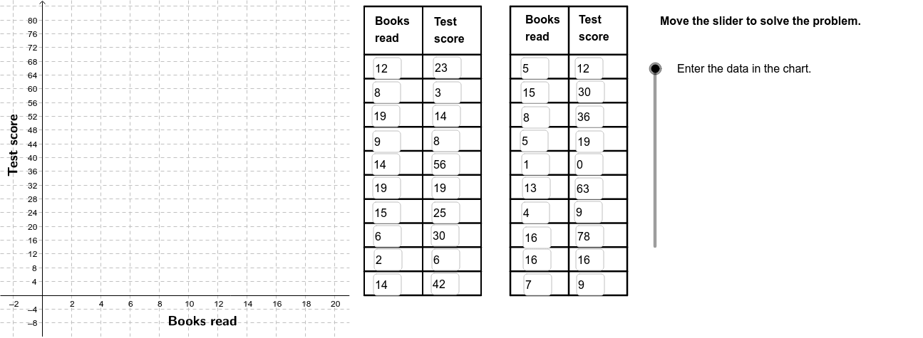
Scatter Plot of Vocabulary vs Reading Frequency with Regression Line
Loading the math board and drawing, please wait…
In collections
CCSS IP Math I Unit 4 Lesson 3
① This example demonstrates how to create a scatter plot of students' vocabulary size versus reading frequency and fit a linear regression line to reveal the correlation trend. ② Core mathematical concepts include the Pearson product‑moment correlation coefficient (PMCC), linear regression, scatter‑plot visualization, and interpretation of correlation. ③ Construction highlights: FitLineY draws the regression line, PMCC computes the correlation coefficient, Sequence generates the data points, Segment draws line segments, If and Polygon handle conditional display, RotateText rotates labels, and Textfield enables interactive input. ④ Suitable for high‑school statistics and probability courses, introductory college statistics, and introductory data‑analysis workshops.
GeoGebra Commands & Parameters
FitLineY(PointList1) → LineFitPMCC(PointList1) → CorCoeffTextfield(A2) → InA2Textfield(A3) → InA3Textfield(A4) → InA4Textfield(A5) → InA5Textfield(A6) → InA6Textfield(A7) → InA7Textfield(A8) → InA8Textfield(A9) → InA9Textfield(A10) → InA10Textfield(A11) → InA11Textfield(A12) → InA12Textfield(A13) → InA13Textfield(A14) → InA14Textfield(A15) → InA15Textfield(A16) → InA16Textfield(A17) → InA17Textfield(A18) → InA18Textfield(A19) → InA19Textfield(A20) → InA20Textfield(A21) → InA21Textfield(B2) → InB2Textfield(B3) → InB3Textfield(B4) → InB4Textfield(B5) → InB5Textfield(B6) → InB6Textfield(B7) → InB7Textfield(B8) → InB8Textfield(B9) → InB9Textfield(B10) → InB10Textfield(B11) → InB11Textfield(B12) → InB12Textfield(B13) → InB13Textfield(B14) → InB14Textfield(B15) → InB15Textfield(B16) → InB16Textfield(B17) → InB17Textfield(B18) → InB18Textfield(B19) → InB19Textfield(B20) → InB20Textfield(B21) → InB21Sequence(Segment[(22, 0 + (7 * i)), (30, 0 + (7 * i))], i, 0, 10) → Linesh1Sequence(Segment[(32, 0 + (7 * i)), (40, 0 + (7 * i))], i, 0, 10) → Linesh2Sequence(Segment[(22 + (4 * i), 0), (22 + (4 * i), 84)], i, 0, 2) → Linesv1Sequence(Segment[(32 + (4 * i), 0), (32 + (4 * i), 84)], i, 0, 2) → Linesv2Segment((22, 84), (30, 84)) → top1Segment((32, 84), (40, 84)) → top2If(LineVisible, "Hide Best Fit Line", "Show Best Fit Line") → LineButtonPolygon((21, y(Corner[1])), Corner[2], Corner[3], (21, y(Corner[4]))) → poly1, a, b, c, dRotateText("Books read", 0) → BottomLegendIf(CorVisible, "Hide Correlation Coefficient", "Show Correlation Coefficient") → CorButtonRotateText("Test score", 90*°) → SideLegend
AI Drawing Prompt Reference
Create a scatter plot showing the relationship between students' vocabulary size and reading frequency, with a linear regression line to reveal the correlation trend. Include axes, tick marks, grid lines, and a title for clear visualization of data points and the regression line. Use text fields for data input and conditional statements to control the display of certain elements. Start by drawing the axes and grid, then generate data points and fit the regression line, finally adding text fields and labels.
The prompt above was compiled from the original drawing commands and is for reference only.