Sampling Distributions: Dynamic Visualization of Sample Statistics

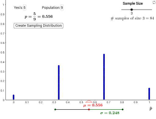
This interactive GeoGebra example demonstrates the concept of sampling distributions by repeatedly drawing samples from a population of blue and non-blue items, then plotting the distribution of sample statistics (such as sample proportion or mean) using dot plots. It illustrates how the sampling distribution emerges from many random samples, connecting to the central limit theorem, expected value, hypothesis testing, and the binomial distribution. The construction uses commands like Sequence to generate multiple samples, Join and DotPlot to display the statistics, Textfield and sliders to control sample size and number of samples, Mean, SD, and Binomial for calculations, and Polygon and Segment to visualize the population and sample subsets. This resource is ideal for high school or introductory college statistics courses, helping students grasp how sample statistics vary and how their distribution approximates normality with larger sample sizes, while also supporting discussions on hypothesis testing and p-values.