
Rolling Parabola with Parametric Curve Locus
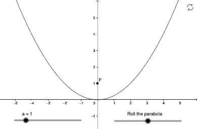
Loading the math board and drawing, please wait…
This example demonstrates how a “rolling parabola” can be visualized by generating a curve that traces the evolving shape/feature as the configuration moves continuously. It focuses on representing the rolling motion through a parameter (t) and converting the motion constraints into a Cartesian curve. The main mathematical ideas are parametric/coordinate-geometry modeling, the locus (trajectory) concept, and the geometric interpretation of a function-defined curve such as a parabola. Construction is carried out in GeoGebra using CurveCartesian to create the curve (object a, with parameter t, and parameters/controls b and F), together with supporting objects and labeling (text1) to reflect the current configuration and resulting traced curve. Suitable for high school to early undergraduate learners studying functions, analytic geometry, and dynamic geometry visualizations.
GeoGebra Commands & Parameters
CurveCartesian((a / sqrt(1 + t^(2)) * ((2 * u) + (t * u^(2)) - t + (sqrt(1 + t^(2)) * asinh(t)))), (a * (u - t)^(2) / sqrt(1 + t^(2))), u, -10, 10) → b
AI Drawing Prompt Reference
Draw a Cartesian parametric locus curve that visualizes a “rolling parabola” by tracing its evolving feature as a configuration parameter t changes. Define the curve using coordinates given by two functions of parameters u and t: x(u,t)=a/sqrt(1+t^2)·(2u+t·u^2−t+sqrt(1+t^2)·asinh(t)) and y(u,t)=a·(u−t)^2/sqrt(1+t^2). Treat u as the curve parameter and generate the curve for u ranging from -10 to 10. Use a as a scaling factor and let t control the rolling configuration, then display the resulting traced curve.
The prompt above was compiled from the original drawing commands and is for reference only.