
Relation to Green's Theorem
Loading the math board and drawing, please wait…
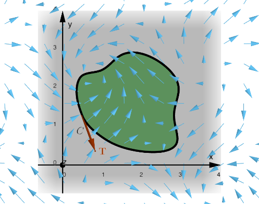
This example demonstrates the relationship with Green's Theorem. Key mathematical concepts include vector fields, line integrals, and area calculation. Using GeoGebra commands like Spline, Tangent, Vector, etc., complex geometric shapes are constructed. Suitable for university calculus courses.
GeoGebra Commands & Parameters
Spline({A, B, C, D, E, F, G, H, I, J, K, A}, 3) → cPoint(c, t) → PTangent(P, c) → tangOrthogonalLine(P, tang, xOyPlane) → perpCircle(P, 1, xOyPlane) → cirIntersect(perp, cir, 1) → Q1Intersect(perp, cir, 2) → Q2Vector(P, Q1) → uVector(P, Q2) → vTranslate(Vector[(0, 0, 1)], P) → kElement(vdir, faces) → SelectVecLaTeX(faces, true, true) → text1Intersect(tang, cir, 1) → P1Intersect(tang, cir, 2) → P2Vector(P, P1) → tvectorSequence(k, k, -1.5, 5.2, xstep) → LxSequence(k, k, -1.5, 5.2, ystep) → LyZip(Zip[Vector[(j, k), (j + (scale * fx(j, k)), k + (scale * fy(j, k)))], j, Lx], k, Ly) → vectorFieldSequence(c(i), i, 0, 1, 0.01) → LMPolygon(LM) → PDTranslate(Vector[(0, 0, 1)], L) → nVector
AI Drawing Prompt Reference
Draw a graph demonstrating the relationship between vector fields and Green's Theorem, featuring a spline curve through nine points. From points on the curve, draw tangent and perpendicular lines, creating two intersection points. Draw vectors from the curve's starting point to these intersections. On the xy-plane, draw a circle intersecting the perpendicular lines at two points, and draw vectors from the starting point to these intersection points. Finally, create a vector field on the plane with a series of vectors and represent the integral region with a polygon formed by the curve.
The prompt above was compiled from the original drawing commands and is for reference only.