
Quadratic Function Graph and Properties
Loading the math board and drawing, please wait…
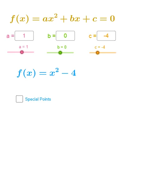
This GeoGebra example demonstrates the graph of a quadratic function y = ax² + bx + c, highlighting its vertex, axis of symmetry, roots (zeros), and discriminant. The core mathematical concepts include quadratic function characteristics, the quadratic formula, and the relationship between functions and equations. The construction uses commands such as Expand to expand expressions, Root to find roots, Extremum to locate extrema, Segment to draw line segments, Textfield and input boxes (CasillaDeEntrada) for user input, If and Sequence for conditional and sequential operations, Append and TableText to generate tables, and sliders for dynamic parameter adjustment. It is suitable for high school students learning quadratic functions, solving quadratic equations, and exploring graph transformations, and can be used for classroom demonstrations or independent student exploration.
GeoGebra Commands & Parameters
Expand((a * x^(2)) + (b * x) + c) → fRoot(f) → A, BSegment(P, C) → hTextfield(xP) → CasillaDeEntrada1Textfield(a) → CasillaDeEntrada2Textfield(b) → CasillaDeEntrada3Textfield(c) → CasillaDeEntrada4If(e ≟ x_v, l1_b, l1_a) → l2Sequence(f(l2(i)), i, 1, Length[l2]) → l3Append(x, l2) → lxAppend(y, l3) → lyTableText(Append[x, l2], Append[y, l3], "c_|v") → texto15Textfield(b) → CasillaDeEntrada3_{1}Textfield(c) → CasillaDeEntrada4_{1}Textfield(b) → CasillaDeEntrada3_{2}Textfield(c) → CasillaDeEntrada4_{2}Textfield(b_{1}) → CasillaDeEntrada3_{3}Textfield(c_{1}) → CasillaDeEntrada4_{3}Textfield(b_{2}) → CasillaDeEntrada3_{4}Textfield(c_{2}) → CasillaDeEntrada4_{4}Sequence((l2(k), l3(k)), k, 1, Length[l2]) → l1Extremum(f) → D
AI Drawing Prompt Reference
Plot the quadratic function y=ax^2+bx+c. Construct the curve from the expression, and mark the two roots (x-intercepts), the vertex, and the axis of symmetry. Provide adjustable/input parameters a, b, and c so the curve and root locations update when values change. Draw a connecting segment related to the vertex and corresponding position. Collect root-related coordinates to form a small table with the header c_|v, and also indicate the extremum point of the function to highlight its key properties.
The prompt above was compiled from the original drawing commands and is for reference only.