
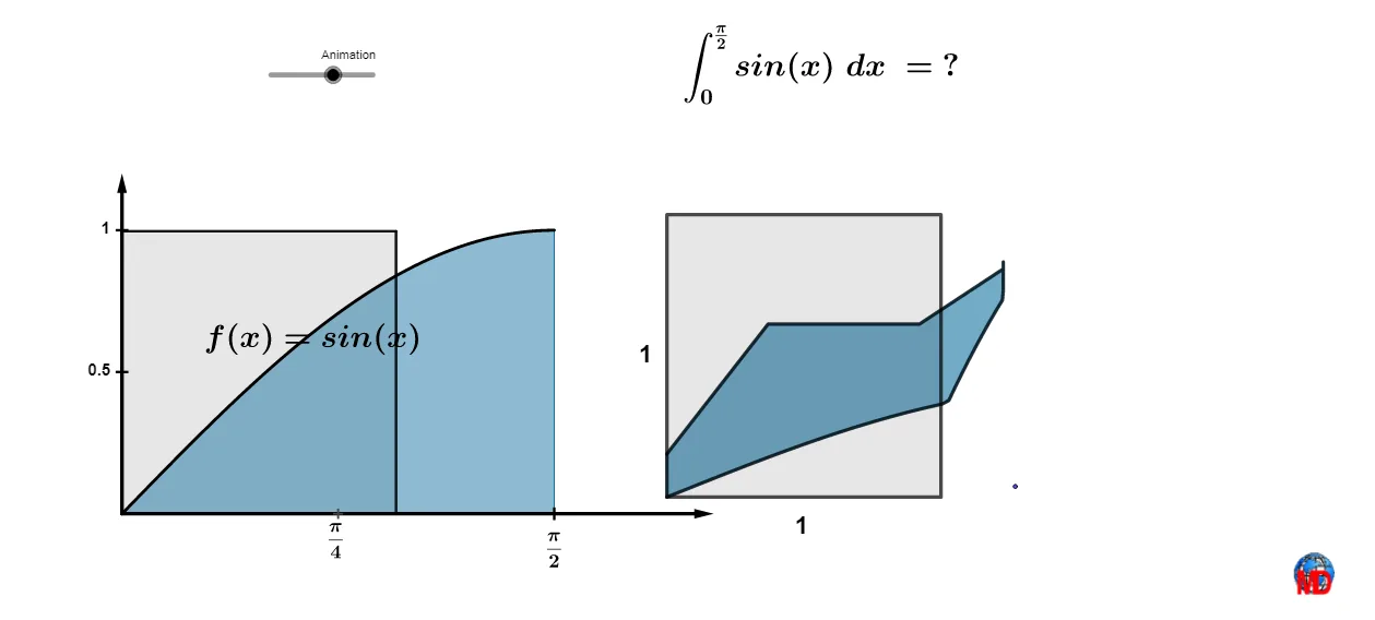
Proof without words: Integral of sin(x) between 0 and pi/2
Loading the math board and drawing, please wait…
This example demonstrates the calculation process of the integral of sin(x) between 0 and pi/2 through geometric visualization. Key math concepts include integral calculus, trigonometric functions, and geometric shapes. GeoGebra commands/objects used in the construction are Polygon, Sequence, Midpoint, Join, Integral, Point, Length, Vector, Translate, PolyLine, Centroid, Line, and Intersect. Suitable for high school and above students to learn and understand the fundamental theorem of calculus.
GeoGebra Commands & Parameters
Polygon(I, J, 4) → poly1, g, h, i, j, K, LSequence(Translate[I, Vector[(i * Vector[I, J])]], i, 0, 1, 1 / n) → l2Midpoint(K, I) → NJoin(Sequence[Rotate[l2, i, N], i, 0, (2 * π), (2 * π / 4)]) → l3Sequence((i, f(i)), i, 0, π / 2, 1 / n) → l1Sequence(Translate[M, Vector[(i * Vector[M, O])]], i, 0, 1, 1 / 16) → l1bSequence(Translate[O, Vector[(i * Vector[O, (0, 0)])]], i, 0, 1, 1 / 20) → l1cJoin({l1, l1b, l1c}) → l6Sequence(Vector[Element[l6, i], Element[l3, i]], i, 1, Length[l3]) → l4Sequence(Translate[Element[l6, i], Vector[(Animation / 10 * Element[l4, i])]], i, 1, Length[l6]) → l5Polygon(A, B, C, D) → poly4, a, b, c, dIntegral(f, 0, 1.5707963267948966) → ePoint(poly4) → EPolygon(l5) → poly2Length(l3) → lLength(l6) → kVector((0, 0), I) → uPolygon(P, E, 4) → poly3, m, q, r, s, Q, RTranslate(poly3, Vector[(Animation / 10 * u)]) → poly3'PolyLine(l5) → tCentroid(poly3') → SLine(S, yAxis) → f_1Intersect(f_1, poly3') → T, ULine(S, xAxis) → g_1Intersect(g_1, poly3') → V, WVector((0, 0), (0, 1.2)) → vVector((0, 0), (2.15, 0)) → wMidpoint(P, O) → Z
AI Drawing Prompt Reference
Draw a geometric proof figure showing the integral of sine from 0 to pi/2. Start with a square, rotate and copy it four times to form a symmetric pattern. Generate points along the sine curve on the axes, translate these points to match the rotated square vertices, and connect corresponding points with line segments to create a dynamic grid. Add a rectangle representing the integral area, and place a rotated square inside it, drawing horizontal and vertical lines through its center to intersect the rectangle edges, illustrating area relationships. The overall composition visualizes the integral through curves, grids, and geometric shapes.
The prompt above was compiled from the original drawing commands and is for reference only.