Anatomy of a Logarithmic Function: Special Points and Riemann-Sum Geometry (Part

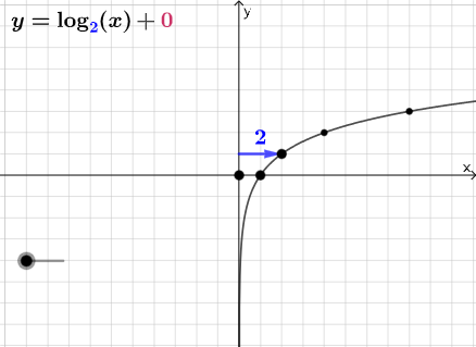
This GeoGebra example visually “dissects” a logarithmic function by highlighting its structural behavior near key points and connecting the idea of accumulated area to upper/lower sums (Riemann sums) and related geometric partitions. The core topics are logarithmic functions and their graphs, special points used to anchor the construction, linear functions as auxiliary references, and the geometric interpretation of upper and lower sums / Riemann sums. Construction is driven by GeoGebra commands such as Point (to place key vertices like interval endpoints and reference markers), Intersect (to compute intersection points that tie auxiliary lines/curves to the log graph), and Vector (to encode directional relationships needed for connecting, partitioning, or measuring geometric quantities). The presence of many labeled intermediate objects and text annotations indicates a step-by-step, concept-first build that makes the relationship between the log curve’s shape and area-sum approximations more tangible. Suitable for high school to early university instruction, especially function graphing and pre-calculus/intro-calculus lessons about area and Riemann sums.