Power Functions with Equilateral Triangles and Linear Equations

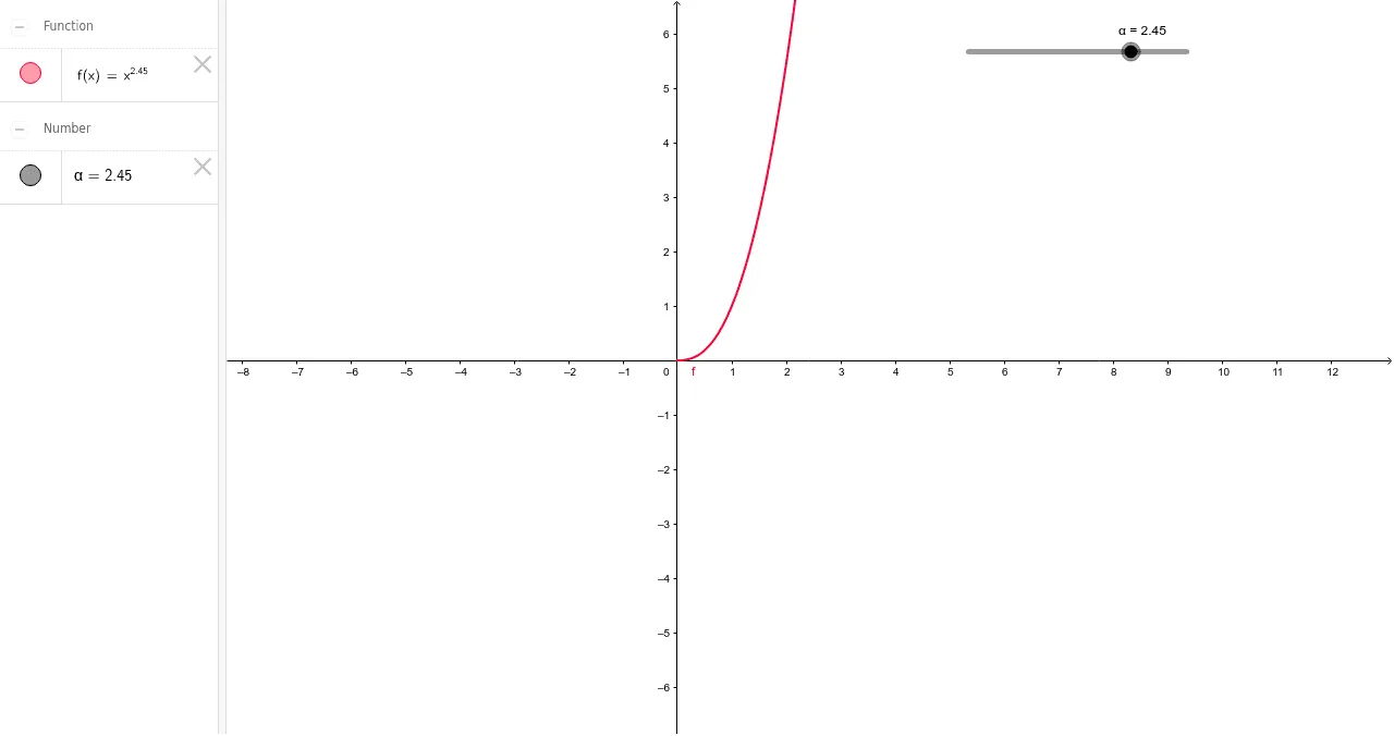
This GeoGebra example demonstrates power functions (y = x^α) and their graphical representation, intertwined with equilateral triangles, linear equations, and combinatorial concepts. The core mathematical concepts include the definition and graph characteristics of power functions, such as how the exponent α affects the curve's shape (parabolas, hyperbolas, cubic curves, etc.), geometric properties of equilateral triangles, linear functions and their equations, and basic combinatorial counting principles. Construction highlights: based on the summary, the example uses objects α and f, likely with a slider for α to dynamically change the exponent, and a function f to plot the power curve. It may also incorporate equilateral triangles and linear equations as additional visual elements, utilizing GeoGebra commands for function input, sliders, and geometric object creation. This resource is suitable for high school or early college students to explore how power function graphs vary with parameters, and to see interdisciplinary connections between algebra, geometry, and combinatorics. It can serve as a classroom demonstration or a self-guided exploration tool.