
Polyhedra with Extreme Vertex Distributions on a Sphere
Loading the math board and drawing, please wait…
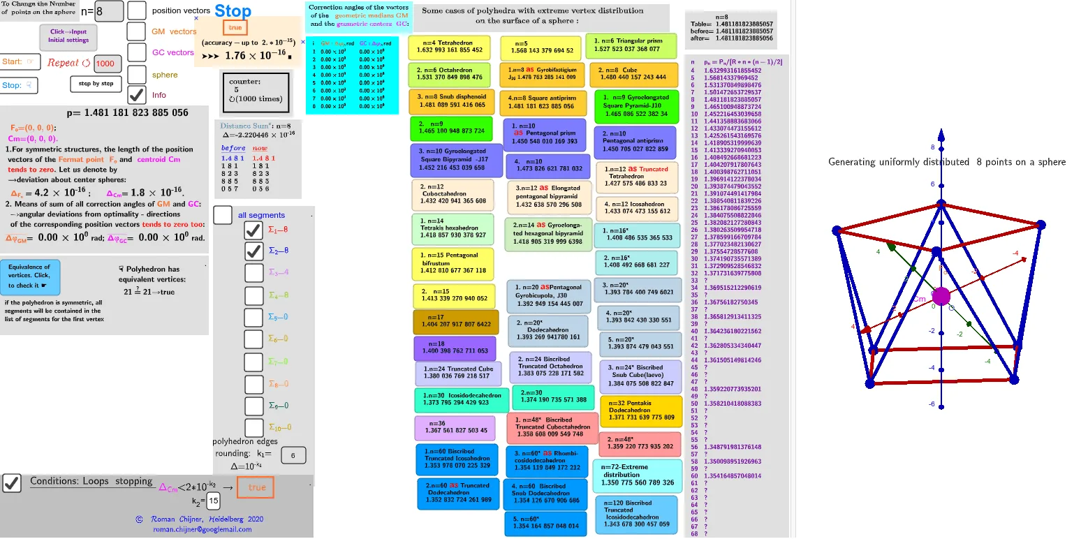
① This example demonstrates polyhedra whose vertices are distributed in extreme ways on the surface of a sphere, such as clustering or spreading, and explores their geometric properties. ② Core mathematical concepts include polyhedra, spherical geometry, centroid/barycenter, optimization problems, linear programming, matrices and vectors, and combinations of equilateral and scalene triangles. ③ Construction highlights: using GeoGebra commands such as Sphere, Text/LaTeX, TableText, Append/Zip/If/Sum, and UnicodeToLetter, along with objects like m1, Um1, Wii_Pc, lP', and sliders/input boxes (InputBox) to adjust parameters n, r, i0 for dynamic exploration. ④ Suitable for high school to university-level mathematics, especially for advanced teaching in solid geometry, optimization, and computational geometry, as well as for mathematical modeling or competition training.
GeoGebra Commands & Parameters
Text("" + Um1) → txt_pLaTeX(Um1) → lll1_1LaTeX(Um0) → lll0Sphere(O, R) → p1Textfield(n) → InputBox1Textfield(i0) → InputBox2Text(r) → TxtrTextfield(k_1) → InputBox4UnicodeToLetter(34) → u34Textfield(k_2) → InputBox5TableText(ltxt0, ltxt1, "v") → textltxt01Append(A, Sequence[((random(), random(), random()) * R), i, 2, n]) → l2sText(("(up\; to\; 10^{-15})\;\\ accuracy= " * ScientificText[cc, 3]), C, true, true) → text5rZip(Vector[a, a + UnitVector[a]], a, lP') → lVector1Textfield(scale) → InputBox6TableText(Append["i", 1…n], Append[" \fgcolor{orange}{GM :Δφ_i}, rad", l1], Append["\fgcolor{magenta}{GC :Δφ_i} , rad", l1c], "v") → text23If(bu, "Animation", "Stop") → bue0Zip(Vector[a, a + (1.5 * UnitVector[b])], a, lP', b, Wi_P) → lVector3Zip(Vector[a, a + (1.5 * UnitVector[b])], a, lP', b, Wi_Pc) → lVector2TableText({Join[{{"n"}, Sequence[i, i, 4, 69 + 3]}], Join[{{" p_n=P_n/[R*n*(n-1)/2]"}, lp}]}, "vl") → txt_lpSum(Flatten[Sequence[Append[Sequence[Element[txt_p, i], i, m1(k), m2(k)], " "], k, 1, 5]]) → txtUm1Text("\;\;\;\;\;\;\;\;\;\;\;\;\;\fgcolor{" + (If[c', "orange", "brown"]) + "} \boxed{ " + c' + ("}\;\;\;\; \;\;\;\;\; \\\;\; ( accuracy- up\; to\;\; 2.*10^{" - k_2) + ("\;})\;\\\;\; ➤➤➤\;\;\;\scalebox{1.5}{ " + (ScientificText[cc, 3])) + "}\;█ ", C, true, true) → text9Zip(Segment[Element[lP', y(a)], Element[lP', z(a)]], a, ll1bb(1)) → ll1Zip(Segment[Element[lP', y(a)], Element[lP', z(a)]], a, ll1bb(2)) → ll2Zip(Segment[Element[lP', y(a)], Element[lP', z(a)]], a, ll1bb(3)) → ll3Zip(Segment[Element[lP', y(a)], Element[lP', z(a)]], a, ll1bb(4)) → ll4
AI Drawing Prompt Reference
Create a 3D sphere centered at O with radius R, then add several styled text labels (including LaTeX-style formulas and a highlighted boxed expression). Generate n points on or near the sphere using random coordinates scaled by R, but controlled by parameters such as r and i0 so the vertex distribution exhibits extreme behavior (clustering or spreading). Include an on-figure accuracy statement and auxiliary parameter text. Connect relevant point pairs with line segments to form the main geometric structure, and display symbolic table entries, including color-coded annotations for GM:Δφ_i and GC:Δφ_i with units in radians, so the piecewise angular increments are visually indicated.
The prompt above was compiled from the original drawing commands and is for reference only.