
Polar Rose Curves: r = a·cos(bθ) and r = a·sin(bθ) with Dynamic Construction
Loading the math board and drawing, please wait…
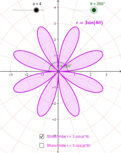
① This example demonstrates the classic polar rose curves defined by r = a·cos(bθ) or r = a·sin(bθ), showing how the number and shape of petals change as parameters a and b vary. ② Core mathematical concepts include polar coordinates, trigonometric periodicity, parametric representation, symmetry, and the relationship between the integer b and petal count (b petals if b is odd, 2b petals if b is even). ③ Construction details: The GeoGebra commands include CurveCartesian to plot the polar equation in Cartesian parametric form, along with sliders for a, b, and θ; points A and B, lines, and angle objects are used to visualize the radius r as θ changes, with text labels text1 and text2 displaying the equation and parameters. ④ This is suitable for high school or early college courses in analytic geometry, trigonometry, or pre-calculus, and serves as an interactive tool for exploring polar graphs and parametric curves.
GeoGebra Commands & Parameters
CurveCartesian((r(i) * cos(i)), (r(i) * sin(i)), i, 0, θ) → bPoint(b) → ACurveCartesian(cos(i), sin(i), i, 0, 6.283185307179586) → cLine((0, 0), (1, 1)) → eLine((0, 0), (1, 1.7320508075688772)) → fLine((0, 0), (1.7320508075688772, 1)) → gLine((0, 0), (-1.73205, 1)) → hLine((0, 0), (1, -1.73205)) → iLine((0, 0), (1, -1)) → jLine((0, -0.02), (0.9659258262890683, 0.23881904510252072)) → kLine((0, 0), (0.25881904510252074, 0.9659258262890683)) → lLine((0, -0.02), (-0.25881904510252085, 0.9659258262890683)) → mLine((0, -0.02), (-0.9659258262890682, 0.258819045102521)) → nCurveCartesian((2 * cos(i)), (2 * sin(i)), i, 0, 6.28319) → oCurveCartesian((3 * cos(i)), (3 * sin(i)), i, 0, 6.28319) → pCurveCartesian((4 * cos(i)), (4 * sin(i)), i, 0, 6.28319) → qCurveCartesian((5 * cos(i)), (5 * sin(i)), i, 0, 6.28319) → sCurveCartesian((6 * cos(i)), (6 * sin(i)), i, 0, 6.28319) → tCurveCartesian((7 * cos(i)), (7 * sin(i)), i, 0, 6.28319) → uCurveCartesian((v(i) * cos(i)), (v(i) * sin(i)), i, 0, θ) → wLine(A, B) → dAngle(xAxis, d) → α
AI Drawing Prompt Reference
Draw polar rose curves defined by r = a·cos(bθ) and r = a·sin(bθ), where a and b are adjustable parameters. Use sliders to change the values of a and b and observe how the number and shape of petals change. Plot sine and cosine curves from 0 to 2π to visualize how the radius r varies with angle θ.
The prompt above was compiled from the original drawing commands and is for reference only.