Polar Equations Grapher: Dynamic Exploration of Polar Curves

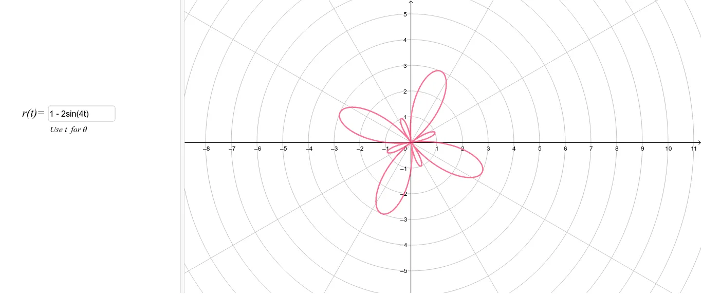
This GeoGebra example demonstrates how to interactively graph polar equations using an input box, allowing users to visualize how different polar functions produce distinct curves. The core mathematical concepts include the relationship between polar and Cartesian coordinates, the dependence of radial distance on angle, and the geometric properties of classic polar curves such as roses, spirals, and circles. Construction highlights: the example uses a Textfield for user input, the CurveCartesian command to convert polar equations into parametric Cartesian form, and variables like t, f, and a to control parameters and plotting range, with text1 and text2 displaying the current equation and instructions. This resource is suitable for high school or early college mathematics, helping students grasp the polar coordinate system, the effect of parameters on curve shapes, and the power of dynamic software for function visualization.