
Polar Grapher
Loading the math board and drawing, please wait…
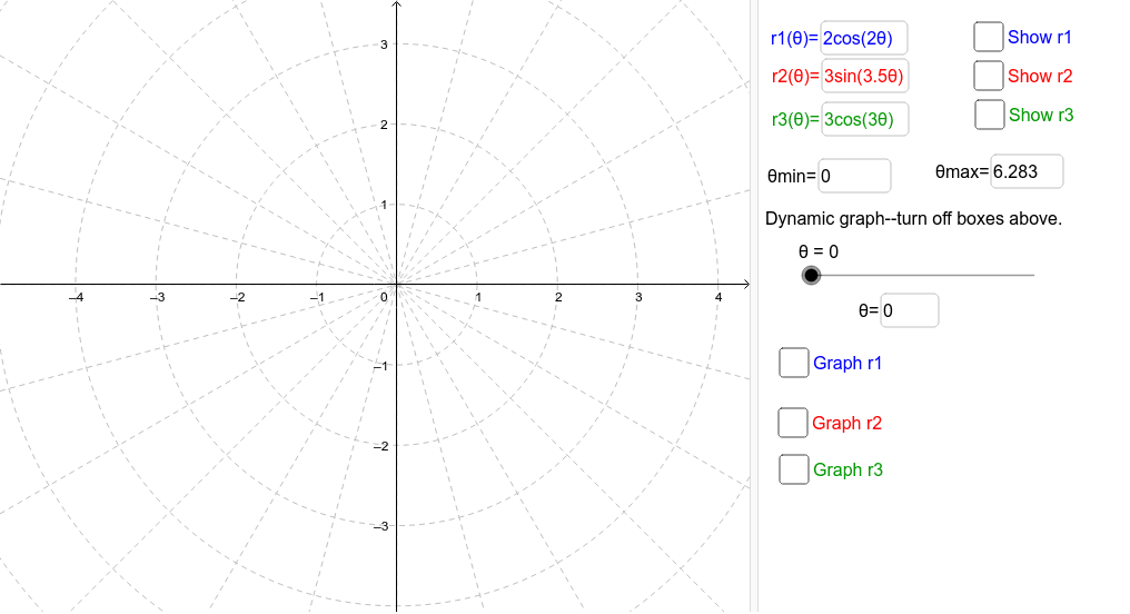
This example demonstrates how to use GeoGebra to draw polar graphs. It covers basic concepts in the polar coordinate system, such as radius and angle. By inputting different polar coordinate equations, various shapes can be observed. Main commands used include CurveCartesian and Textfield, suitable for high school mathematics education and learning.
GeoGebra Commands & Parameters
CurveCartesian((r1(t) * cos(t)), (r1(t) * sin(t)), t, θmin, θmax) → aCurveCartesian((r2(t) * cos(t)), (r2(t) * sin(t)), t, θmin, θmax) → bTextfield(r1) → r1InputTextfield(r2) → r2InputTextfield(θmin) → ΘminTextfield(θmax) → ΘmaxCurveCartesian((r3(t) * cos(t)), (r3(t) * sin(t)), t, θmin, θmax) → cTextfield(r3) → r3InputCurveCartesian((r1(t) * cos(t)), (r1(t) * sin(t)), t, θmin, θ) → a1CurveCartesian((r3(t) * cos(t)), (r3(t) * sin(t)), t, θmin, θ) → c1CurveCartesian((r1(t) * cos(t)), (r1(t) * sin(t)), t, θmin, θmax) → a2CurveCartesian((r2(t) * cos(t)), (r2(t) * sin(t)), t, θmin, θmax) → b2CurveCartesian((r3(t) * cos(t)), (r3(t) * sin(t)), t, θmin, θmax) → c2CurveCartesian((r2(t) * cos(t)), (r2(t) * sin(t)), t, θmin, θ) → b1Textfield(θ) → ThetaEquals