
Polar Graph Exploration
Loading the math board and drawing, please wait…
In collections
BC Calculus
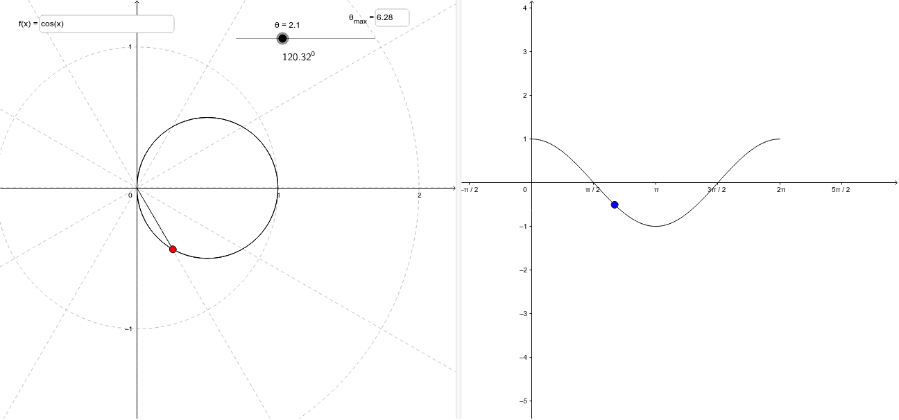
This example explores the relationship between rectangular and polar coordinate systems, helping students understand the basic concepts of polar graphs. Key mathematical concepts include polar coordinates, conversion between rectangular and polar coordinates, and parametric equations. Using GeoGebra commands such as Segment, CurveCartesian, and Function, the dynamic process of drawing polar graphs is demonstrated. Suitable for high school mathematics education, particularly in coordinate geometry and trigonometry.
GeoGebra Commands & Parameters
Segment(E, P) → dCurveCartesian(f(t) * cos(t), f(t) * sin(t), t, 0, 6.283185307179586) → cTextfield(f) → inputBox1Function(f, 0, 6.283185307179586) → gTextfield(max) → inputBox2
AI Drawing Prompt Reference
Create a dynamic illustration showing the relationship between polar and Cartesian coordinates, featuring input fields for a function expression and maximum polar value, generating a polar curve from the function, demonstrating the conversion process with line segments, and displaying the corresponding Cartesian function graph.
The prompt above was compiled from the original drawing commands and is for reference only.