
Polar Derivatives in Cartesian Coordinates
Loading the math board and drawing, please wait…
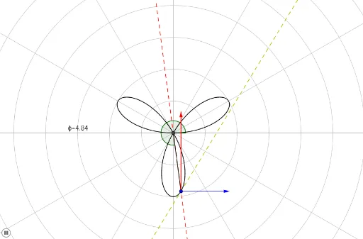
This example demonstrates the geometric interpretation and calculation of derivatives of polar equations in Cartesian coordinates (x, y). Key math concepts include polar-to-Cartesian conversion, the geometric meaning of derivatives, and vector operations. GeoGebra commands/objects used in construction are OrthogonalLine, Intersect, Segment, Point, Line, Angle, CurveCartesian, and Vector. Suitable for high school and above students to understand the practical application and visualization of polar derivatives.
GeoGebra Commands & Parameters
OrthogonalLine(A, xAxis) → gIntersect(g, xAxis) → BSegment(A, B) → hIntersect(xAxis, yAxis) → DSegment(D, C) → iPoint(xAxis) → ELine(D, C) → jAngle(E, D, F) → αCurveCartesian(((f(u) * cos(u)), (f(u) * sin(u))), u, ϕ_{low}, ϕ_{high}) → aVector(C, G) → uVector(C, H) → v
AI Drawing Prompt Reference
Draw the geometric interpretation and calculation of derivatives of polar equations in Cartesian coordinates. Start by drawing the x-axis and y-axis, then draw a perpendicular line from the origin to the x-axis, marking the foot of the perpendicular and the intersection with the x-axis. Next, draw a line segment from the origin to the foot of the perpendicular, and another line segment from an arbitrary point on the x-axis to the origin. Then, plot a polar curve, and draw vectors from the origin to points on the curve to demonstrate vector operations and the geometric meaning of derivatives.
The prompt above was compiled from the original drawing commands and is for reference only.