
Polar Curve Intersections Demo
Loading the math board and drawing, please wait…
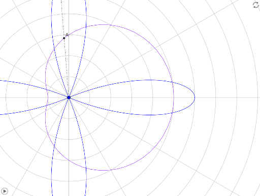
This example demonstrates the calculation and visualization of intersections between two polar curves. It involves core mathematical concepts such as polar coordinate equations, function graphing, and intersection solving. Key GeoGebra commands used include CurveCartesian for Cartesian plotting, Textfield and Ray for text and ray creation, with parameters like n, r, r_1, r_2 for dynamic interaction. Suitable for high school mathematics education to understand polar coordinate systems and function intersection properties.
GeoGebra Commands & Parameters
CurveCartesian((r_1(θ); θ), θ, 0, (2 * 3.141592653589793)) → r_+CurveCartesian((r_2(θ); θ), θ, 0, (2 * 3.141592653589793)) → bTextfield(r) → InputBox1CurveCartesian((p_1(θ); θ), θ, 0, (2 * 3.141592653589793)) → BCurveCartesian((p_2(θ); θ), θ, 0, (2 * 3.141592653589793)) → dTextfield(p) → InputBox2Ray(D, A) → fRay(D, C) → g
AI Drawing Prompt Reference
Draw two polar curves defined by adjustable polar equations, and display their intersection points. Include two input boxes to adjust the parameters in these equations. From the intersection point, draw two rays extending outward to highlight the intersection and its directions. The figure demonstrates the concept of polar curve intersections for educational purposes.
The prompt above was compiled from the original drawing commands and is for reference only.