
Point-by-Point Graphing of Polynomial Functions
Loading the math board and drawing, please wait…
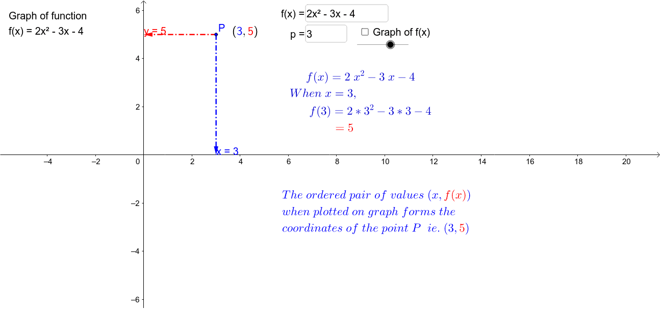
This example demonstrates how to graph a function by plotting points, illustrating that the graph is the set of ordered pairs (x, y) where y = f(x). Key math concepts include function definition, polynomial function properties, and coordinate geometry. It utilizes GeoGebra commands and objects such as Coefficients, Length, Sequence, Join, Element, RemoveUndefined, Textfield, and CoordinatePointeronAxisToolNew for construction. Suitable for high school mathematics education to understand the formation of function graphs and the plotting of polynomial functions.
GeoGebra Commands & Parameters
Coefficients(f) → list1Length(list1) → n_tSequence(h(x)^(k), k, n_t - 1, 2, -1) → list2Join({list2, list2a}) → list2sumSequence(Element[list1, n] * Element[list2sum, n], n, 1, n_t - 1) → list3uElement(list1, n_t) → h_cRemoveUndefined(Sequence[If[abs(Element[list1, n]) > 0, Element[list3u, n], ""], n, 1, n_t - 1]) → list3Length(list3) → n_{list3}Textfield(f) → inputBox1Textfield(p) → inputBox2CoordinatePointeronAxisToolNew(P) → text4, text5, u, v, text6
AI Drawing Prompt Reference
Plot a polynomial function graph by point-by-point method. First define the function f, then calculate its coefficients, generate the sequence of each term's coefficient, and finally plot the polynomial function graph based on these coefficients.
The prompt above was compiled from the original drawing commands and is for reference only.