
Plotting Colored Parametric Surfaces with Trace Method
Loading the math board and drawing, please wait…
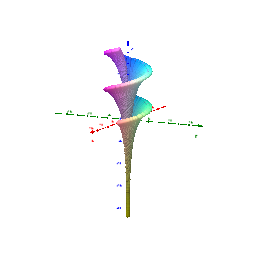
This example demonstrates how to plot colored parametric surfaces using the trace method. Key mathematical concepts include parametric equations and color mapping. The construction involves commands such as Sequence, Join, Zip, RemoveUndefined, Max, Min, Surface, CurveCartesian, Textfield, and Point. Suitable for high school and above students or teachers for teaching or research on the visualization of parametric surfaces.
GeoGebra Commands & Parameters
Sequence(Sequence[(u_{min} + (i * dx), v_{min} + (j * dy)), i, 0, Na], j, 0, Na) → l1aJoin(l1a) → uvZip(fz(a, b), a, u0, b, v0) → Z1Zip(fy(a, b), a, u0, b, v0) → Y1Zip(fx(a, b), a, u0, b, v0) → X1RemoveUndefined(X1) → X1EMax(X1E) → x1maxaMin(X1E) → x1minaRemoveUndefined(Y1) → Y1EMax(Y1E) → x2maxaMin(Y1E) → x2minaRemoveUndefined(Z1) → Z1EMax(Z1E) → x3maxaMin(Z1E) → x3minaSurface((((r_X * 5) * cos(u)) * sin(v)), (((r_Y * 5) * sin(u)) * sin(v)), ((r_Z * 5) * (cos(v) + log(tan(v / 2)))) + (1.3 * u), u, u_{min}, u_{max}, v, v_{min}, v_{max}) → hCurveCartesian((fx(t, a_v) * r_X), (fy(t, a_v) * r_Y), (fz(t, a_v) * r_Z), t, u_{min}, u_{max}) → f_uCurveCartesian((fx(a_u, t) * r_X), (fy(a_u, t) * r_Y), (fz(a_u, t) * r_Z), t, v_{min}, v_{max}) → f_vTextfield(u_{min}) → inputBox4Textfield(u_{max}) → inputBox5Textfield(v_{min}) → inputBox6Textfield(v_{max}) → inputBox7Textfield(Pstyle) → Textfeld1Textfield(Nx) → Textfeld2Textfield(v_u) → Textfeld3Textfield(v_v) → Textfeld4Textfield(r_X) → inputBox8Textfield(r_Y) → inputBox9Textfield(r_Z) → inputBox10Point(f_u, 0) → Pr_{0}Point(f_u, 0.02) → Pr_{1}Point(f_u, 0.04) → Pr_{2}Point(f_u, 0.06) → Pr_{3}Point(f_u, 0.08) → Pr_{4}Point(f_u, 0.1) → Pr_{5}Point(f_u, 0.12) → Pr_{6}Point(f_u, 0.14) → Pr_{7}Point(f_u, 0.16) → Pr_{8}Point(f_u, 0.18) → Pr_{9}Point(f_u, 0.2) → Pr_{10}Point(f_u, 0.22) → Pr_{11}Point(f_u, 0.24) → Pr_{12}Point(f_u, 0.26) → Pr_{13}Point(f_u, 0.28) → Pr_{14}Point(f_u, 0.3) → Pr_{15}Point(f_u, 0.32) → Pr_{16}Point(f_u, 0.34) → Pr_{17}Point(f_u, 0.36) → Pr_{18}Point(f_u, 0.38) → Pr_{19}Point(f_u, 0.4) → Pr_{20}Point(f_u, 0.42) → Pr_{21}Point(f_u, 0.44) → Pr_{22}Point(f_u, 0.46) → Pr_{23}Point(f_u, 0.48) → Pr_{24}Point(f_u, 0.5) → Pr_{25}Point(f_u, 0.52) → Pr_{26}Point(f_u, 0.54) → Pr_{27}Point(f_u, 0.56) → Pr_{28}Point(f_u, 0.58) → Pr_{29}Point(f_u, 0.6) → Pr_{30}Point(f_u, 0.62) → Pr_{31}Point(f_u, 0.64) → Pr_{32}Point(f_u, 0.66) → Pr_{33}Point(f_u, 0.68) → Pr_{34}Point(f_u, 0.7) → Pr_{35}Point(f_u, 0.72) → Pr_{36}Point(f_u, 0.74) → Pr_{37}Point(f_u, 0.76) → Pr_{38}Point(f_u, 0.78) → Pr_{39}Point(f_u, 0.8) → Pr_{40}Point(f_u, 0.82) → Pr_{41}Point(f_u, 0.84) → Pr_{42}Point(f_u, 0.86) → Pr_{43}Point(f_u, 0.88) → Pr_{44}Point(f_u, 0.9) → Pr_{45}Point(f_u, 0.92) → Pr_{46}Point(f_u, 0.94) → Pr_{47}Point(f_u, 0.96) → Pr_{48}Point(f_u, 0.98) → Pr_{49}Point(f_u, 1) → Pr_{50}Point(f_v, 0) → Pr_{51}Point(f_v, 0.02) → Pr_{52}Point(f_v, 0.04) → Pr_{53}Point(f_v, 0.06) → Pr_{54}Point(f_v, 0.08) → Pr_{55}Point(f_v, 0.1) → Pr_{56}Point(f_v, 0.12) → Pr_{57}Point(f_v, 0.14) → Pr_{58}Point(f_v, 0.16) → Pr_{59}Point(f_v, 0.18) → Pr_{60}Point(f_v, 0.2) → Pr_{61}Point(f_v, 0.22) → Pr_{62}Point(f_v, 0.24) → Pr_{63}Point(f_v, 0.26) → Pr_{64}Point(f_v, 0.28) → Pr_{65}Point(f_v, 0.3) → Pr_{66}Point(f_v, 0.32) → Pr_{67}Point(f_v, 0.34) → Pr_{68}Point(f_v, 0.36) → Pr_{69}Point(f_v, 0.38) → Pr_{70}Point(f_v, 0.4) → Pr_{71}Point(f_v, 0.42) → Pr_{72}Point(f_v, 0.44) → Pr_{73}Point(f_v, 0.46) → Pr_{74}Point(f_v, 0.48) → Pr_{75}Point(f_v, 0.5) → Pr_{76}Point(f_v, 0.52) → Pr_{77}Point(f_v, 0.54) → Pr_{78}Point(f_v, 0.56) → Pr_{79}Point(f_v, 0.58) → Pr_{80}Point(f_v, 0.6) → Pr_{81}Point(f_v, 0.62) → Pr_{82}Point(f_v, 0.64) → Pr_{83}Point(f_v, 0.66) → Pr_{84}Point(f_v, 0.68) → Pr_{85}Point(f_v, 0.7) → Pr_{86}Point(f_v, 0.72) → Pr_{87}Point(f_v, 0.74) → Pr_{88}Point(f_v, 0.76) → Pr_{89}Point(f_v, 0.78) → Pr_{90}Point(f_v, 0.8) → Pr_{91}Point(f_v, 0.82) → Pr_{92}Point(f_v, 0.84) → Pr_{93}Point(f_v, 0.86) → Pr_{94}Point(f_v, 0.88) → Pr_{95}Point(f_v, 0.9) → Pr_{96}Point(f_v, 0.92) → Pr_{97}Point(f_v, 0.94) → Pr_{98}Point(f_v, 0.96) → Pr_{99}Point(f_v, 0.98) → Pr_{100}Point(f_v, 1) → Pr_{101}Textfield(fx) → inputBox1Textfield(fy) → inputBox2Textfield(fz) → inputBox3
AI Drawing Prompt Reference
Draw a colored parametric surface defined by x = r_X·5·cos(u)·sin(v), y = r_Y·5·sin(u)·sin(v), z = r_Z·5·(cos(v)+ln(tan(v/2)))+1.3·u. Show two families of parameter curves on the surface (constant‑v curves in u and constant‑u curves in v) and place a series of equally spaced trace points along one u‑curve. Provide interactive input fields for u_min, u_max, v_min, v_max, r_X, r_Y, and r_Z to adjust the domain and scaling.
The prompt above was compiled from the original drawing commands and is for reference only.