Plot the Rotation about Origin

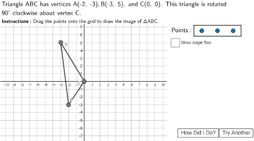
① This example demonstrates how to dynamically plot a triangle rotated about the origin by a specified angle, showing both the original and rotated figures and their coordinate changes. ② Core mathematical concepts include rotation transformation in the Cartesian plane, rotation angle, coordinate mapping of corresponding points, and rotation invariance (side lengths and angles remain unchanged). ③ Construction highlights: from the construction summary, it uses Polygon to draw the original triangle ABC, Rotate to generate the rotated triangle A1B1C1, and Angle, Segment, Ray to mark the rotation angle and corresponding sides; a slider (rotangle) controls the rotation angle, with Point, Circle and other objects providing interactive feedback. ④ Suitable for upper middle school or high school geometry and coordinate geometry lessons, as well as for students to explore rotation rules and understand the geometric meaning of coordinate formulas.