
Picard's Method of Successive Approximations
Loading the math board and drawing, please wait…
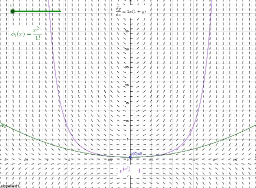
This example demonstrates Picard's method of successive approximations, an iterative method for solving initial value problems. It involves core concepts of differential equations. Using commands like SlopeField and Sum, the construction of successive approximations is illustrated. Suitable for university-level calculus courses.
GeoGebra Commands & Parameters
SlopeField(((2 * x) * (y + 1))) → slopefield1Sum(t^((2 * n)) / n!, n, 1, k) → ϕ_k
AI Drawing Prompt Reference
Create a diagram illustrating Picard's method of successive approximations. First, draw a slope field on the coordinate plane for the differential equation y' = 2x(y+1), shown as short line segments whose slopes vary with x and y. Then, overlay a curve representing the k-th approximation, given by the sum from n=1 to k of t^(2n)/n!. This curve starts from the initial point and approaches the exact solution as k increases. The diagram should clearly show the relationship between the slope field and the approximation curve, with the curve superimposed on the field to demonstrate the iterative approximation process.
The prompt above was compiled from the original drawing commands and is for reference only.