
Logistic Models of COVID-19 in Vermont Over Time
Loading the math board and drawing, please wait…
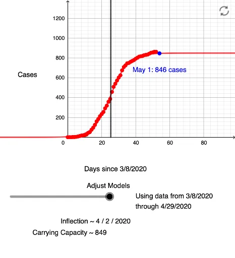
① This interactive example demonstrates how logistic models fit the cumulative COVID-19 case data in Vermont, USA, over time, showing the growth curve and its saturation. ② Core mathematical concepts include the logistic function, data fitting, sequences, and the use of rays for auxiliary visualization, blending statistics with function modeling. ③ Construction highlights: GeoGebra commands such as Sequence to generate data series, FitLogistic to fit the logistic curve to case data, and Ray to draw auxiliary lines; numerous objects (e.g., D54, B54) are used to represent data points and curve elements. ④ Suitable for high school to college-level mathematics or statistics courses, this example aids in understanding epidemic modeling, curve fitting, and real-world data visualization, and can support discussions on mathematical analysis of pandemic trends.
GeoGebra Commands & Parameters
Sequence(l1(k), k, 1, n) → l3FitLogistic(l3) → Cases_{VT}Ray((b, 0), (b, 1)) → gRay((b, 0), (b, 1)) → g_{copy}
AI Drawing Prompt Reference
Create a scatter plot showing cumulative COVID-19 cases over time, with time on the x-axis and case counts on the y-axis. Plot discrete data points for actual observations, then fit a smooth S-shaped logistic growth curve that rises slowly, accelerates, and eventually plateaus. Add a vertical auxiliary ray extending upward from a point on the x-axis to mark the current observation time. The graph should emphasize the contrast between raw data points and the fitted curve, illustrating the epidemic's growth and saturation.
The prompt above was compiled from the original drawing commands and is for reference only.