
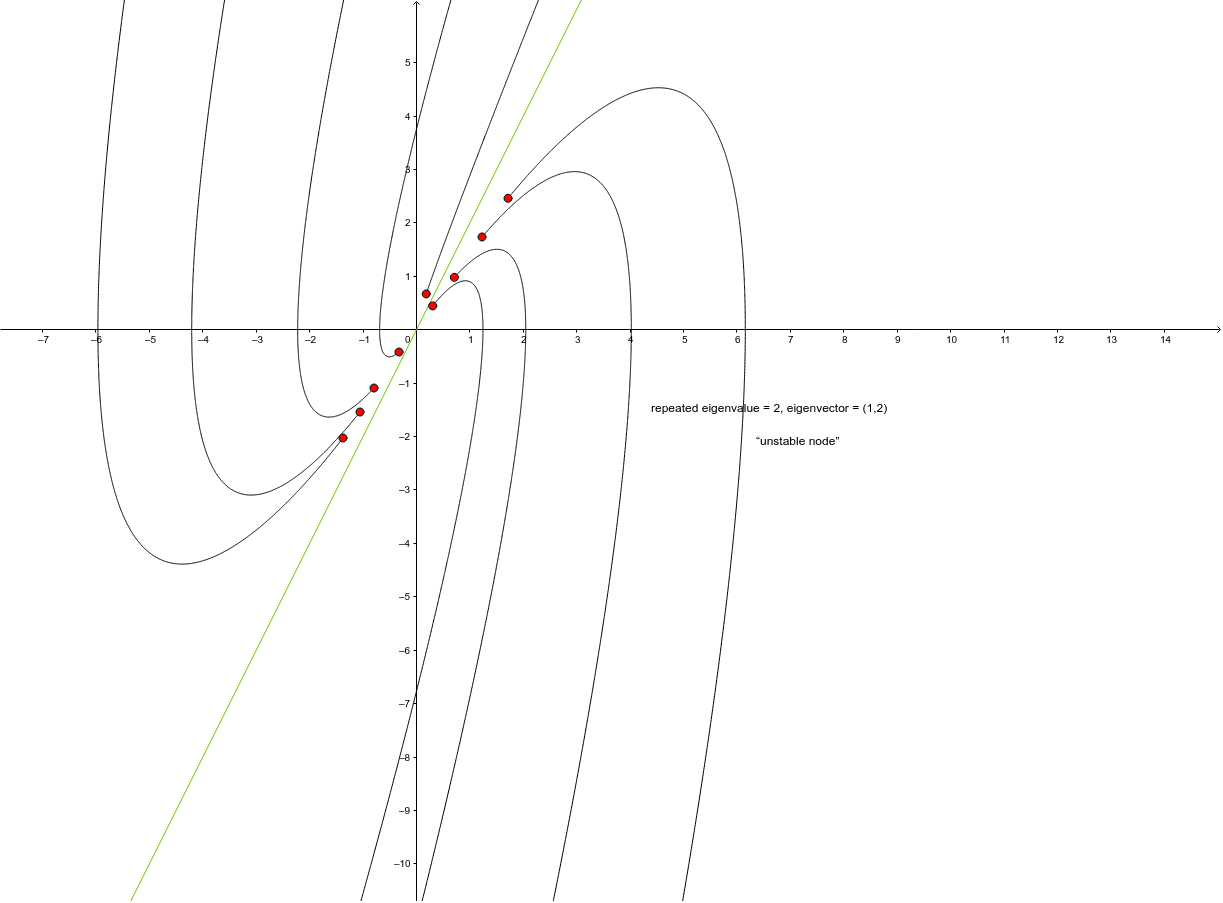
Phase Portrait of Linear DE System with Real Repeated Eigenvalues
Loading the math board and drawing, please wait…
In collections
Differential Equations
This example demonstrates the phase portrait for a linear system of differential equations with constant coefficients featuring two real, repeated eigenvalues. Key math concepts include linear differential equations, eigenvalues and eigenvectors, phase portraits, and stability analysis. Construction highlights involve commands like SolveODE for solving ODEs, Intersect for finding intersections, and Line for plotting tangent lines. Suitable for university-level mathematics and differential equations courses to visually understand system dynamics under repeated eigenvalue conditions.
GeoGebra Commands & Parameters
SolveODE(g, f, x(A), y(A), 10, 0.001) → numericalIntegral1SolveODE(g, f, x(D), y(D), 10, 0.001) → numericalIntegral2SolveODE(g, f, x(E), y(E), 10, 0.001) → numericalIntegral3SolveODE(g, f, x(B), y(B), 10, 0.001) → numericalIntegral4SolveODE(g, f, x(C), y(C), 10, 0.001) → numericalIntegral5SolveODE(g, f, x(G), y(G), 10, 0.001) → numericalIntegral7SolveODE(g, f, x(H), y(H), 10, 0.001) → numericalIntegral6SolveODE(g, f, x(F), y(F), 10, 0.001) → numericalIntegral8SolveODE(g, f, x(I), y(I), 10, 0.001) → numericalIntegral9Intersect(xAxis, yAxis) → JLine(J, K) → a
AI Drawing Prompt Reference
Draw the phase portrait of a linear system of differential equations with real repeated eigenvalues. Show system trajectories including several paths starting from the origin, and mark the intersection point of the x-axis and y-axis. Draw lines from this intersection to points on the trajectories to indicate tangent directions. The graph should clearly illustrate the system dynamics and stability characteristics under repeated eigenvalue conditions.
The prompt above was compiled from the original drawing commands and is for reference only.