
Phase Plane
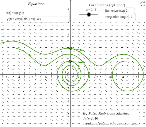
Loading the math board and drawing, please wait…
This example demonstrates the phase plane of differential equations, visualizing system dynamics through vector fields and trajectories. Core math concepts include differential equations, vector fields, trajectories, and isoclines. Construction highlights the use of GeoGebra commands/objects like SlopeField, Textfield, SolveODE, Vector, UnitVector, and ImplicitCurve. Suitable for university students in mathematics, physics, and related fields studying dynamic systems.
GeoGebra Commands & Parameters
SlopeField(v(x, y) / u(x, y), N, l, xmin, ymin, xmax, ymax) → slopefield1Textfield(u) → InputBox1Textfield(v) → InputBox2SolveODE(v(x, y) / u(x, y), x(A), y(A), tmin, numStep) → fAbackSolveODE(v(x, y) / u(x, y), x(A), y(A), tmax, numStep) → fAforwSolveODE(v(x, y) / u(x, y), x(B), y(B), tmin, numStep) → fBbackSolveODE(v(x, y) / u(x, y), x(B), y(B), tmax, numStep) → fBforwVector((u(x(B), y(B)), v(x(B), y(B)))) → VBUnitVector(VA) → vAUnitVector(VB) → vBVector(A, A + vA) → v_AVector(B, B + vB) → v_BImplicitCurve(u(x, y)) → IsoclineXImplicitCurve(v(x, y)) → IsoclineYTextfield(numStep) → InputBox3Textfield(tmax) → InputBox4