
Slope Field Plotter
Loading the math board and drawing, please wait…
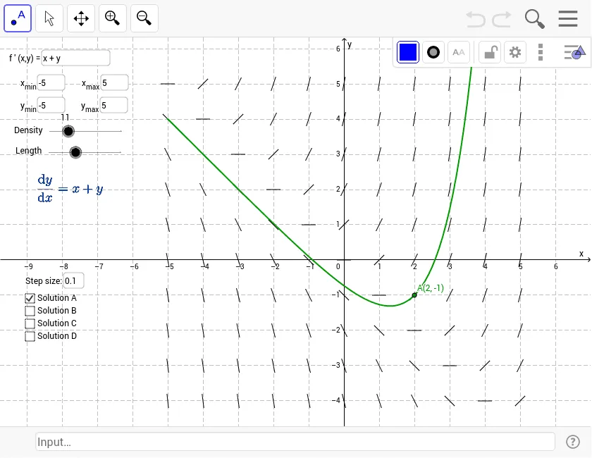
This example demonstrates how to plot a direction field for a specified differential equation and optionally display particular solutions. Core math concepts include differential equations, direction fields, and particular solutions. It uses GeoGebra commands/objects like Textfield, SlopeField, SolveODE. Suitable for high school students and teachers.
GeoGebra Commands & Parameters
Textfield(f) → inputBox1Textfield(x_{min}) → inputBox2Textfield(x_{max}) → inputBox3Textfield(y_{min}) → inputBox4Textfield(y_{max}) → inputBox5SlopeField(f, n, L, x_{min}, y_{min}, x_{max}, y_{max}) → slopefield1Textfield(delta) → inputBox6SolveODE(f, x(A), y(A), x_{max}, delta) → numericalIntegral1SolveODE(f, x(A), y(A), (-x_{max}), delta) → numericalIntegral2SolveODE(f, x(B), y(B), x_{max}, delta) → numericalIntegral3SolveODE(f, x(B), y(B), x_{min}, delta) → numericalIntegral4SolveODE(f, x(C), y(C), x_{max}, delta) → numericalIntegral5SolveODE(f, x(C), y(C), x_{min}, delta) → numericalIntegral6SolveODE(f, x(D), y(D), x_{max}, delta) → numericalIntegral7SolveODE(f, x(D), y(D), x_{min}, delta) → numericalIntegral8
AI Drawing Prompt Reference
Plot a direction field for a given differential equation and display several particular solutions. First, input the differential equation and the display range for the direction field, then draw the field. Next, plot several solution curves passing through different initial points based on given conditions to show the behavior and trends of the solutions over time.
The prompt above was compiled from the original drawing commands and is for reference only.