
Pear Curves
Loading the math board and drawing, please wait…
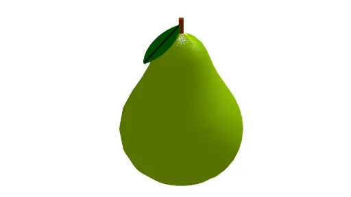
This example demonstrates the construction and 3D visualization of pear curves. It involves core mathematical concepts such as quadratic equations, cosine functions, rotation, symmetry, and solid geometry. Key GeoGebra commands and objects used in the construction include Spline, Rotate, Surface, Circle, Cylinder, Sequence, Mirror, Point, Segment, PointIn, Line, and CircumcircleArc. It is suitable for high school students and mathematics enthusiasts exploring complex curves and 3D shapes.
GeoGebra Commands & Parameters
Spline(l1, 3) → aRotate(a, 90°, xAxis) → a'Surface(a', (2 * π), zAxis) → bRotate(A, 90°, xAxis) → A'Circle(A' - (0, 0, 0.2), 0.1, zAxis) → cCylinder(c, 0.7665838069903629) → d, e, fRotate(J, 90°, xAxis) → J'Sequence(Rotate[J' + (0.4, 0, 0.05), i, zAxis], i, 0, (2 * π), (2 * π / 6)) → l2Sequence(Rotate[J' + (0.02, 0, 0.05), i, zAxis], i, 0, (2 * π), (2 * π / 12)) → l3Sequence(Polygon[Element[l3, i], Element[l3, i + 1], Element[l2, i]], i, 1, Length[l3]) → l4Mirror(a, yAxis) → a'_1Point(yAxis) → KSegment(A, K) → gPointIn(f) → LSegment(L, M) → hPoint(h) → NLine(N, yAxis) → iPoint(i) → OCircumcircleArc(L, O, M) → kMirror(k, h) → k'