
Particle Polarity Exchanger V1.1: Dynamic 3D Geometry Demo
Loading the math board and drawing, please wait…
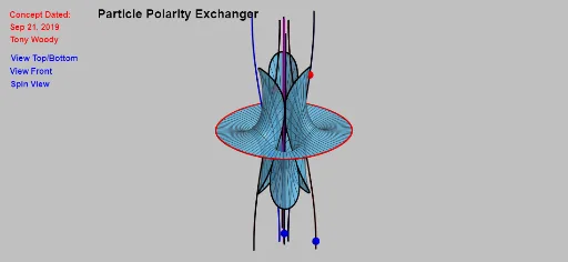
① This example demonstrates a dynamic 3D geometric system called 'Particle Polarity Exchanger', where sliders and buttons control the exchange of particle polarity, showing spatial curves, surfaces, and vector relationships. ② Core mathematical concepts include 3D vectors, ellipses, distributions, frequency distributions, and parametric equations of spatial curves and surfaces, involving geometric transformations such as midpoint, distance, rotation, and reflection. ③ Construction highlights: uses GeoGebra commands like Surface, CurveCartesian, Sequence, Segment, Midpoint, Line, Distance, Circle, Length, Ray, Mirror, Point, If, Rotate, Corner, and builds objects such as a, n, eV, sV, surface_1, curves, segments, circles, rays, points, with interactive buttons and sliders. ④ Suitable for high school to university level mathematics teaching, to understand 3D geometric constructions, parametric equations, and dynamic transformations, also useful as an example for mathematical modeling or computer-aided geometric design.
GeoGebra Commands & Parameters
Surface(((-cos(t))) / r - (r^((2 * n) + 1) / ((2 * n) + 1) * cos((((2 * n) + 1) * t))), ((-sin(t))) / r - (r^((2 * n) + 1) / ((2 * n) + 1) * sin((((2 * n) + 1) * t))), ((((-a)) / n * r^(n)) * cos((n * t))), r, sV, eV, t, 0, (2 * π)) → surface_1CurveCartesian(((-cos(t))) / eV - (eV^((2 * n) + 1) / ((2 * n) + 1) * cos((((2 * n) + 1) * t))), ((-sin(t))) / eV - (eV^((2 * n) + 1) / ((2 * n) + 1) * sin((((2 * n) + 1) * t))), ((((-a)) / n * eV^(n)) * cos((n * t))), t, 0, (2 * π)) → curve_{id}CurveCartesian(((-cos(t))) / sV - (sV^((2 * n) + 1) / ((2 * n) + 1) * cos((((2 * n) + 1) * t))), ((-sin(t))) / sV - (sV^((2 * n) + 1) / ((2 * n) + 1) * sin((((2 * n) + 1) * t))), ((((-a)) / n * sV^(n)) * cos((n * t))), t, 0, (2 * π)) → curve_{od}Sequence(Segment[curve_{id}((i * π / 4)), curve_{od}((i * π / 4))], i, 1, 7, 2) → liste1Segment(A, B) → segABMidpoint(segAB) → CLine((0, 0, 1), (0, 0, -1)) → axis_{z}Distance(Pnt_{Or2}, B) → dist_{B}Distance(Pnt_{Or1}, A) → dist_{A}Circle(Origin, dist_{A} - dist_{B}, axis_{z}) → circle_1Segment(Origin, C) → segOCLength(curve_{id}, 0, (2 * π)) → length_bLength(curve_{od}, 0, (2 * π)) → length_dRay(A, B) → rayABCurveCartesian(((-cos(t_t))) / r - (r^((2 * n) + 1) / ((2 * n) + 1) * cos((((2 * n) + 1) * t_t))), ((-sin(t_t))) / r - (r^((2 * n) + 1) / ((2 * n) + 1) * sin((((2 * n) + 1) * t_t))), ((((-a)) / n * r^(n)) * cos((n * t_t))), r, sV, eV) → circle_{02}Mirror(A, axis_{z}) → A'Point(rayAB) → EIf(z(E) ≟ z(A'), 1, 0) → zeroSlopeLength(circle_{02}, sV, eV) → length_e2Segment(A, B_2) → gLine((0, 0, 1), (0, 0, -1)) → hPoint(h) → FCurveCartesian(((0, 0, 6) * (1 - t)^(3)) + (((0, 0, 3) * t) * (1 - t)^(2)) + (((0, 0, -3) * t^(2)) * (1 - t)) + ((0, 0, -6) * t^(3)), t, 0, 1) → curve_{bezier1}CurveCartesian(((0.25, 0, 6) * (1 - t)^(3)) + (((0.5, 0, 5) * t) * (1 - t)^(2)) + (((5.5, 0, -5) * t^(2)) * (1 - t)) + ((1.75, 0, -6) * t^(3)), t, 0, 1) → curve_{bezier2}Mirror(curve_{bezier2}, Origin) → curve_{bezier6}Rotate(curve_{bezier2}, (-(120°)), axis_{z}) → curve_{bezier4}Rotate(curve_{bezier2}, (-(240°)), axis_{z}) → curve_{bezier3}Mirror(curve_{bezier3}, Origin) → curve_{bezier7}Mirror(curve_{bezier4}, Origin) → curve_{bezier5}Point(curve_{bezier7}) → Pnt_{bezier7}Point(curve_{bezier6}) → Pnt_{bezier6}Point(curve_{bezier2}) → Pnt_{bezier2}Point(curve_{bezier4}) → Pnt_{bezier4}Point(curve_{bezier3}) → Pnt_{bezier3}Point(curve_{bezier5}) → Pnt_{bezier5}Point(curve_{bezier1}) → Pnt_{bezier1}Corner(1) → corner1
AI Drawing Prompt Reference
Create a dynamic 3D geometric demo featuring a parametric surface defined by inner and outer radii and an integer parameter, with two boundary space curves. Connect corresponding points on the two curves with multiple line segments to form a radial structure. Add a segment between two endpoints, take its midpoint, and draw a circle centered at the origin perpendicular to the z-axis, with radius equal to the difference of distances from the endpoints to the origin. From one endpoint, draw a ray and place a point on it, checking if its z-coordinate equals the mirror image of the other endpoint about the z-axis. Also draw several Bezier curves, rotate and mirror them about the z-axis to create a symmetric 3D framework, and place points on each curve. The overall scene combines surfaces, curves, segments, circles, rays, and points, illustrating geometric transformations and dynamic relationships.
The prompt above was compiled from the original drawing commands and is for reference only.