Partial Derivatives Introduction: Visualizing Directional Change with Vectors

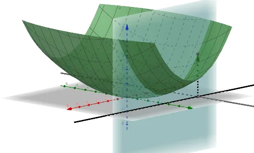
This example demonstrates, in a visually guided way, how a multivariable function’s instantaneous rate of change depends on the chosen direction—capturing the key idea behind partial derivatives. It focuses on core notions such as partial derivatives, the geometric meaning of directional change, and the relationship between tangent-like constructs and local linear behavior. Using GeoGebra, the construction is built around the commands Vector, Line, and Derivative: Vector represents directional information, Line provides the geometric direction/tangent setup at a chosen point, and Derivative is used to compute or display the derivative quantities tied to a specific variable/direction. The construction revolves around objects like f (the function), a, b (base parameters/points), A, B (direction-related points), u (direction/parameter), and additional auxiliary points/parameters (e.g., g, c, d, e, i, k, h, l, j) to organize the configuration and enable the partial-derivative visualization. Suitable for late high school and early college students learning multivariable calculus, especially for building geometric intuition before formal computation.