Normal Distribution: Visualizing the Roles of Mean μ and Standard Deviation σ

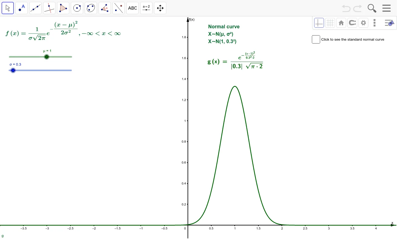
This GeoGebra example dynamically demonstrates how the normal distribution probability density function changes with different values of mean μ (determining the center) and standard deviation σ (determining the spread). The core mathematical concepts include the normal density function, statistical interpretation of mean and standard deviation, and parameter sensitivity of the bell curve. Key construction details: Using the Normal command to plot density curves f and g, employing LaTeX for precise mathematical formulas text1-text6, and incorporating slider 'a' for dynamic parameter adjustment. Ideal for high school and introductory college statistics courses, as well as a visual introduction to the Central Limit Theorem.