
Binomial to Normal Distribution with Gamma Coefficient (Version 2)
Loading the math board and drawing, please wait…
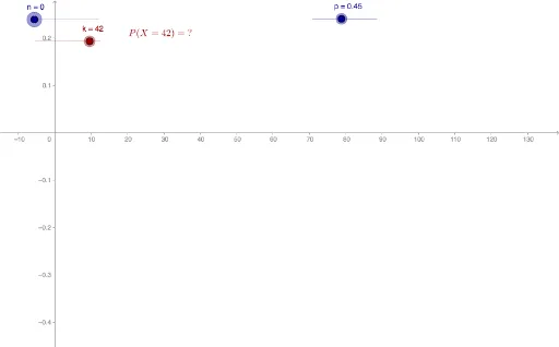
This example demonstrates how a binomial distribution can be transformed into a normal distribution using a gamma coefficient, visualizing the approximation process with piecewise functions and symmetry. It employs GeoGebra commands such as Sequence to generate points, Element to select them, and Segment to draw probability bars and the fitted curve. Interactive sliders for parameters n, p, and the gamma coefficient s allow dynamic exploration, making it suitable for high‑school or university probability and statistics courses, as well as for mathematical modeling and visualization teaching.
GeoGebra Commands & Parameters
Sequence((((gamma(n - 1) / ((gamma((k - (n * p)) / sqrt((n * (p * (1 - p)))) - 1) * gamma(n - (k - (n * p)) / sqrt((n * (p * (1 - p)))) + 1))) * p^((k - (n * p)) / sqrt((n * (p * (1 - p)))))) * (1 - p)^(n - (k - (n * p)) / sqrt((n * (p * (1 - p)))))) * p), k, 0, n) → sSequence((i, Element[s, i + 1]), i, -100, n) → pointsSequence(Segment[Element[points, i + 1], (i, 0)], i, 0, n) → segmentsElement(points, k + 1) → kPointSegment((k, 0), Element[points, k + 1]) → kSeg
AI Drawing Prompt Reference
Draw a dynamic illustration of a binomial distribution with parameters n and p that gradually approaches a normal distribution through a gamma coefficient s. Show probability bars for k = 0 to n whose heights are given by a piecewise formula involving the gamma function, forming a symmetric bell‑shaped curve. Include interactive sliders for n, p, and s so the user can watch the discrete bars smoothly morph into a continuous normal density curve.
The prompt above was compiled from the original drawing commands and is for reference only.