
Normal Distribution Practice Problems
Loading the math board and drawing, please wait…
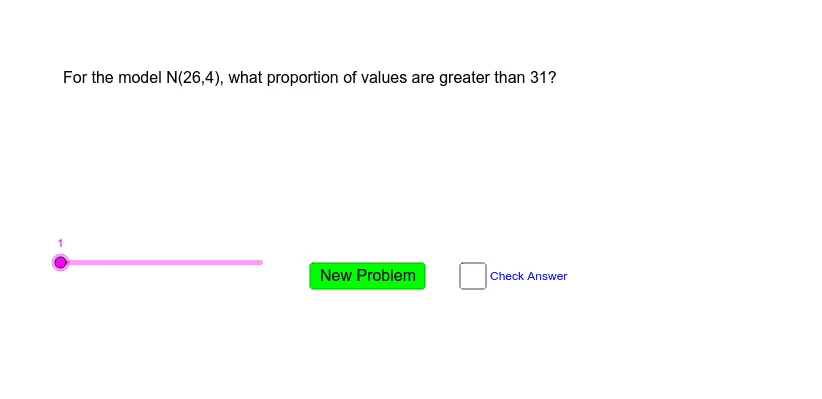
This example demonstrates how to solve typical normal distribution problems involving probability calculations and curve analysis. Key math concepts include normal distribution curves, probability density functions, cumulative distribution functions, standard normal distribution, and integral calculus. It uses GeoGebra commands like Random, Normal, and InverseNormal. Suitable for high school students and above learning probability & statistics.
GeoGebra Commands & Parameters
Random(10, 30) → meanRandom(2, 12) → stdvRandom(mean - (2 * stdv), mean + stdv) → lowerboundRandom(lowerbound + 1, mean + (2 * stdv)) → upperboundNormal(mean, stdv, lowerbound) → lbNormal(mean, stdv, upperbound) → ubRandom(1, 99) → pctileInverseNormal(mean, stdv, pctile / 100) → pctileansInverseNormal(mean, stdv, (50 - pctile / 2) / 100) → bInverseNormal(mean, stdv, (50 + pctile / 2) / 100) → c
AI Drawing Prompt Reference
Draw a normal distribution curve with a mean randomly set between 10 and 30, and a standard deviation randomly set between 2 and 12. Define the lower bound as the mean minus twice the standard deviation, and the upper bound as the mean plus the standard deviation. Calculate the x-value corresponding to a given percentile, and the x-values corresponding to 50% minus and plus half the percentile.
The prompt above was compiled from the original drawing commands and is for reference only.