Normal Distribution Parameter Changes and Interval Probability

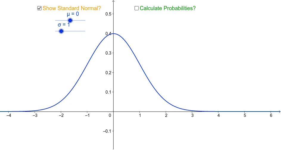
This example demonstrates how changing the mean (μ) and standard deviation (σ) reshapes the normal distribution curve, and how to compute the probability (area under the curve) between two chosen x-values. It focuses on key ideas from probability and calculus: the normal density function, the role of μ shifting the center and σ controlling spread, and the use of definite integrals to obtain interval probabilities. In GeoGebra, the construction relies on creating an integration interval using Segment (to mark lower/upper bounds such as lower, upper and corresponding points like B1/B2), then applying IntegralBetween to the relevant normal density expression with respect to the variable t over [lower, upper]. The objects/parameters (μ, σ, exponent/e-based terms, standardization variable z, and function f) indicate that the model builds the normal pdf formula and evaluates the required area to produce the probability results. Suitable for high school through early undergraduate students studying probability & statistics and introductory calculus, and useful for interactive learning via sliders to connect distribution parameters with computed probabilities.