
Visualizing Binomial Distribution with Normal and Poisson Approximations
Loading the math board and drawing, please wait…
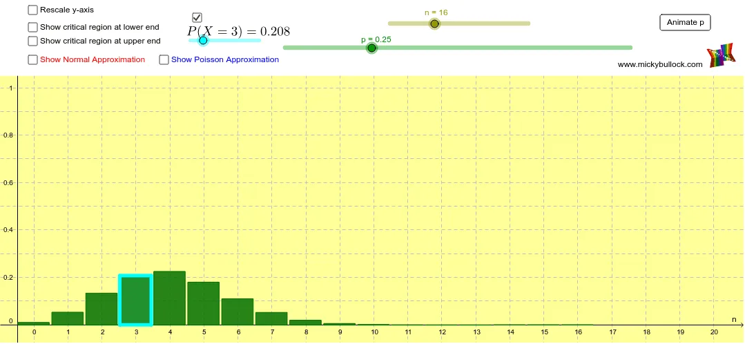
This GeoGebra applet visualizes the Binomial Distribution while allowing interactive control of n and p. It compares the discrete binomial probabilities with continuous approximation curves, highlighting how the Normal approximation and the Poisson approximation perform under different parameter settings. Key concepts include Binomial(n,p), approximating the mean and spread (μ = np, σ = √(np(1−p))) for the Normal curve, using λ = np for the Poisson approximation, and visualizing tail or interval probabilities through accumulated area/region boundaries. The construction uses GeoGebra commands such as Sequence (to generate parameter-dependent indices/ranges), If (to switch behavior near critical boundaries), Sum (to compute discrete probability totals), Integral (to compute areas for the continuous approximation), and Polygon/Line (to draw probability shapes, approximation curves, and dividing lines). Curves are produced by function objects (e.g., f, g, h, i, j) and the app uses objects like μ and σ plus lists (list1–list4) to manage plotting ranges and annotated critical thresholds (criticalhigh/criticallow) driven by sliders. Suitable for secondary school and introductory university courses in probability & statistics, especially for teaching approximation quality and intuition behind tail probabilities.
GeoGebra Commands & Parameters
Sequence(Polygon[(i - 0.475, 0), (i - 0.475, ((Binomial[n, i] * p^(i)) * (1 - p)^(n - i))), (i + 0.45, ((Binomial[n, i] * p^(i)) * (1 - p)^(n - i))), (i + 0.45, 0)], i, 0, n) → list1If(b, Max[list1] / 0.925, 1) → aIf(b, 1, 0) → cPolygon((-2, 1.05), (-2, 1.6), (103, 1.6), (103, 1.05)) → poly1, f, g, h, iSequence(Polygon[(i - 0.475, 0), (i - 0.475, ((Binomial[n, i] * p^(i)) * (1 - p)^(n - i))), (i + 0.45, ((Binomial[n, i] * p^(i)) * (1 - p)^(n - i))), (i + 0.45, 0)], i, 0, criticallow) → list2Sequence(Polygon[(i - 0.475, 0), (i - 0.475, ((Binomial[n, i] * p^(i)) * (1 - p)^(n - i))), (i + 0.45, ((Binomial[n, i] * p^(i)) * (1 - p)^(n - i))), (i + 0.45, 0)], i, criticalhigh, n) → list3Line(A, B) → kIf(n ≤ 20, 20, n) → xmaxSequence(Polygon[(i - 0.475, 0), (i - 0.475, (ℯ^(((-n) * p)) * ((n * p))^(i) / i!)), (i + 0.45, (ℯ^(((-n) * p)) * ((n * p))^(i) / i!)), (i + 0.45, 0)], i, 0, n) → list4Sequence(((Binomial[n, i] * p^(i)) * (1 - p)^(n - i)), i, 0, criticallow) → criticallowsequenceSum(criticallowsequence) → criticallowvalueSequence(((Binomial[n, i] * p^(i)) * (1 - p)^(n - i)), i, criticalhigh, n) → criticalhighsequenceSum(criticalhighsequence) → criticalhighvalueIf(d, criticallow + 1, 0) → criticalhighsliderminPolygon((m - 0.475, 0), (m - 0.475, ((Binomial[n, m] * p^(m)) * (1 - p)^(n - m))), (m + 0.45, ((Binomial[n, m] * p^(m)) * (1 - p)^(n - m))), (m + 0.45, 0)) → poly2, r, s, t, a_1Integral(q, -50, criticallow + 0.5) → criticallownormalIntegral(q, criticalhigh - 0.5, n + 50) → criticalhighnormal
AI Drawing Prompt Reference
Draw a binomial distribution graph by adjusting n and p with sliders. Show the binomial probability bars and approximate curves for normal and Poisson distributions. Set the x-axis maximum to the smaller of n or 20, and mark critical thresholds on the x-axis. Draw binomial probability bars and approximate curves for normal and Poisson distributions, highlighting the regions near the critical thresholds.
The prompt above was compiled from the original drawing commands and is for reference only.