
Normal Distribution by oyunchimegmath
Loading the math board and drawing, please wait…
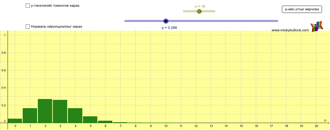
This example demonstrates the normal distribution under the binomial distribution. It involves probability and statistics concepts, constructed using GeoGebra commands such as Sequence, If, Polygon, and Line. Suitable for high school and above students to learn about normal distribution and related knowledge.
GeoGebra Commands & Parameters
Sequence(Polygon[(i - 0.475, 0), (i - 0.475, ((Binomial[n, i] * p^(i)) * (1 - p)^(n - i))), (i + 0.45, ((Binomial[n, i] * p^(i)) * (1 - p)^(n - i))), (i + 0.45, 0)], i, 0, n) → list1If(b, Max[list1] / 0.925, 1) → aIf(b, 1, 0) → cSequence(Polygon[(i - 0.475, 0), (i - 0.475, ((Binomial[n, i] * p^(i)) * (1 - p)^(n - i))), (i + 0.45, ((Binomial[n, i] * p^(i)) * (1 - p)^(n - i))), (i + 0.45, 0)], i, 0, criticallow) → list2Sequence(Polygon[(i - 0.475, 0), (i - 0.475, ((Binomial[n, i] * p^(i)) * (1 - p)^(n - i))), (i + 0.45, ((Binomial[n, i] * p^(i)) * (1 - p)^(n - i))), (i + 0.45, 0)], i, criticalhigh, n) → list3Polygon((-2, 1.05), (-2, 1.6), (maxx + 2, 1.6), (maxx + 2, 1.05)) → poly1, f, g, h, iLine(A, B) → k
AI Drawing Prompt Reference
Draw a binomial distribution probability histogram with n=10 and p=0.5. First, calculate the probability for each i value using the binomial distribution formula and represent it with a polygon. Then, adjust the y-axis maximum based on the value of b. Next, draw a standard normal distribution outline with x-axis range from -2 to 2 and y-axis range from 1.05 to 1.6. Finally, add a line from point A to point B.
The prompt above was compiled from the original drawing commands and is for reference only.